

4.3 An Anisotropic Inverse Problem for Measuring FAWT
89
4.3 An Anisotropic Inverse Problem for Measuring FAWT
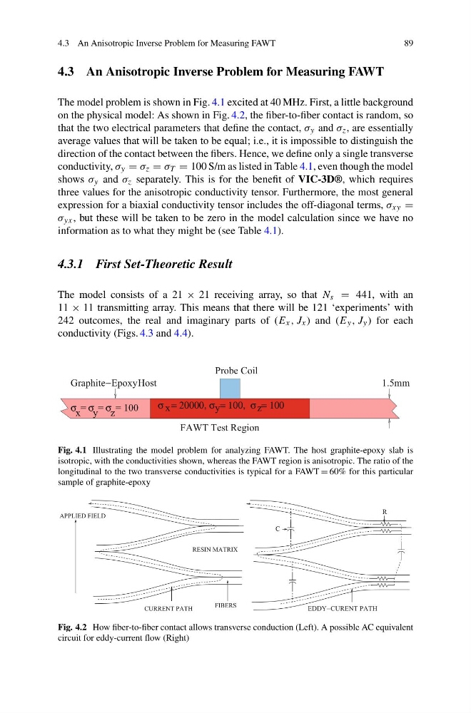
The model problem is shown in Fig. 4.1 excited at 40 MHz. First, a little background
on the physical model: As shown in Fig. 4.2, the fiber-to-fiber contact is random, so
that the two electrical parameters that define the contact, σ y and σ z , are essentially
average values that will be taken to be equal; i.e., it is impossible to distinguish the
direction of the contact between the fibers. Hence, we define only a single transverse
conductivity, σ y = σ z = σ T = 100 S/m as listed in Table 4.1, even though the model
shows σ y and σ z separately. This is for the benefit of VIC-3D®, which requires
three values for the anisotropic conductivity tensor. Furthermore, the most general
expression for a biaxial conductivity tensor includes the off-diagonal terms, σ xy =
σ yx , but these will be taken to be zero in the model calculation since we have no
information as to what they might be (see Table 4.1).
4.3.1 First Set-Theoretic Result
The model consists of a 21 × 21 receiving array, so that N s = 441, with an
11 × 11 transmitting array. This means that there will be 121 ‘experiments’ with
242 outcomes, the real and imaginary parts of (E x , J x ) and (E y , J y ) for each
conductivity (Figs. 4.3 and 4.4).
1.5mm
Graphite−EpoxyHost
σ = 20000, σ = 100, σ = 100
x
y
z
σ x = σ y = σ z = 100
FAWT Test Region
Probe Coil
Fig. 4.1 Illustrating the model problem for analyzing FAWT. The host graphite-epoxy slab is
isotropic, with the conductivities shown, whereas the FAWT region is anisotropic. The ratio of the
longitudinal to the two transverse conductivities is typical for a FAWT = 60% for this particular
sample of graphite-epoxy
APPLIED FIELD
CURRENT PATH
FIBERS
RESIN MATRIX
C
R
EDDY−CURENT PATH
Fig. 4.2 How fiber-to-fiber contact allows transverse conduction (Left). A possible AC equivalent
circuit for eddy-current flow (Right)
89
4.3 An Anisotropic Inverse Problem for Measuring FAWT
The model problem is shown in Fig. 4.1 excited at 40 MHz. First, a little background
on the physical model: As shown in Fig. 4.2, the fiber-to-fiber contact is random, so
that the two electrical parameters that define the contact, σ y and σ z , are essentially
average values that will be taken to be equal; i.e., it is impossible to distinguish the
direction of the contact between the fibers. Hence, we define only a single transverse
conductivity, σ y = σ z = σ T = 100 S/m as listed in Table 4.1, even though the model
shows σ y and σ z separately. This is for the benefit of VIC-3D®, which requires
three values for the anisotropic conductivity tensor. Furthermore, the most general
expression for a biaxial conductivity tensor includes the off-diagonal terms, σ xy =
σ yx , but these will be taken to be zero in the model calculation since we have no
information as to what they might be (see Table 4.1).
4.3.1 First Set-Theoretic Result
The model consists of a 21 × 21 receiving array, so that N s = 441, with an
11 × 11 transmitting array. This means that there will be 121 ‘experiments’ with
242 outcomes, the real and imaginary parts of (E x , J x ) and (E y , J y ) for each
conductivity (Figs. 4.3 and 4.4).
1.5mm
Graphite−EpoxyHost
σ = 20000, σ = 100, σ = 100
x
y
z
σ x = σ y = σ z = 100
FAWT Test Region
Probe Coil
Fig. 4.1 Illustrating the model problem for analyzing FAWT. The host graphite-epoxy slab is
isotropic, with the conductivities shown, whereas the FAWT region is anisotropic. The ratio of the
longitudinal to the two transverse conductivities is typical for a FAWT = 60% for this particular
sample of graphite-epoxy
APPLIED FIELD
CURRENT PATH
FIBERS
RESIN MATRIX
C
R
EDDY−CURENT PATH
Fig. 4.2 How fiber-to-fiber contact allows transverse conduction (Left). A possible AC equivalent
circuit for eddy-current flow (Right)