

72
3 Modeling Composite Structures
-14000
-12000
-10000
-8000
-6000
-4000
-2000
0
2000
4000
0
10 20 30 40 50 60 70 80 90 100
R
Freq(MHz)
25
75
125
-35000
-30000
-25000
-20000
-15000
-10000
-5000
0
5000
0
10 20 30 40 50 60 70 80 90 100
X
Freq(MHz)
25
75
125
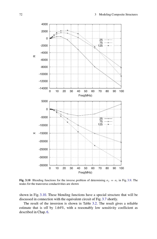
Fig. 3.10 Blending functions for the inverse problem of determining σ y = σ z in Fig. 3.9. The
nodes for the transverse conductivities are shown
shown in Fig. 3.10. These blending functions have a special structure that will be
discussed in connection with the equivalent circuit of Fig. 3.7 shortly.
The result of the inversion is shown in Table 3.2. The result gives a reliable
estimate that is off by 1.64%, with a reasonably low sensitivity coefficient as
described in Chap. 6.
3 Modeling Composite Structures
-14000
-12000
-10000
-8000
-6000
-4000
-2000
0
2000
4000
0
10 20 30 40 50 60 70 80 90 100
R
Freq(MHz)
25
75
125
-35000
-30000
-25000
-20000
-15000
-10000
-5000
0
5000
0
10 20 30 40 50 60 70 80 90 100
X
Freq(MHz)
25
75
125
Fig. 3.10 Blending functions for the inverse problem of determining σ y = σ z in Fig. 3.9. The
nodes for the transverse conductivities are shown
shown in Fig. 3.10. These blending functions have a special structure that will be
discussed in connection with the equivalent circuit of Fig. 3.7 shortly.
The result of the inversion is shown in Table 3.2. The result gives a reliable
estimate that is off by 1.64%, with a reasonably low sensitivity coefficient as
described in Chap. 6.