

3.6 An Anisotropic Inverse Problem for Measuring FAWT
71
It is somewhat easier to predict the variation of a measured signal when the
conductivity of the sample is changed than it is to predict the variation of the signal
when the FAWT is changed. The problem is somewhat simplified if the sample
thickness is known a priori, but knowledge of the sample thickness should not be
a requirement; the information can presumably be extracted from multi-frequency
data. Our model is useful in generating the prediction of signal variation when the
conductivity changes. Another possible method, other than the computer model, for
determining the relationship between conductivity and measured signal would be to
measure the signal given known-conductivity samples. It is unlikely, however, that
we would have enough samples to accurately determine the response to conductivity
change using strictly experimental data. A useful approach might be to use the
model in conjunction with experimental data to determine a better approximation
of the relationship.
3.6 An Anisotropic Inverse Problem for Measuring FAWT
Following the previous discussion of eddy-current detection of prepreg FAWT, we
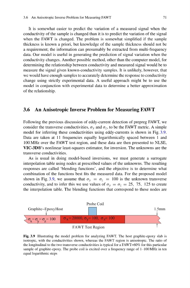
consider the transverse conductivities, σ y and σ z , to be the FAWT metric. A simple
model for inferring these conductivities using eddy-currents is shown in Fig. 3.9.
Data are taken at 11 frequencies equally logarithmically spaced between 1 and
100 MHz over the FAWT test region, and these data are then presented to NLSE,
VIC-3D®’s nonlinear least-squares estimator, for inversion. The unknowns are the
transverse conductivities.
As is usual in doing model-based inversions, we must generate a surrogate
interpolation table using nodes at prescribed values of the unknowns. The resulting
responses are called ‘blending functions’, and the objective is to determine what
combination of the functions best fits the measured data. For the proposed model
shown in Fig. 3.9, we assume that σ y = σ z = 100 is the unknown transverse
conductivity, and to infer this we use values of σ y = σ z = 25, 75, 125 to create
the interpolation table. The blending functions that correspond to these nodes are
1.5mm
Graphite−EpoxyHost
σ = 20000, σ = 100, σ = 100
x
y
z
σ
x
= σ
y
= σ
z
= 100
FAWT Test Region
Probe Coil
Fig. 3.9 Illustrating the model problem for analyzing FAWT. The host graphite-epoxy slab is
isotropic, with the conductivities shown, whereas the FAWT region is anisotropic. The ratio of
the longitudinal to the two transverse conductivities is typical for a FAWT=60% for this particular
sample of graphite-epoxy. The probe coil is excited over a frequency range of 1–100 MHz in ten
equal logarithmic steps
71
It is somewhat easier to predict the variation of a measured signal when the
conductivity of the sample is changed than it is to predict the variation of the signal
when the FAWT is changed. The problem is somewhat simplified if the sample
thickness is known a priori, but knowledge of the sample thickness should not be
a requirement; the information can presumably be extracted from multi-frequency
data. Our model is useful in generating the prediction of signal variation when the
conductivity changes. Another possible method, other than the computer model, for
determining the relationship between conductivity and measured signal would be to
measure the signal given known-conductivity samples. It is unlikely, however, that
we would have enough samples to accurately determine the response to conductivity
change using strictly experimental data. A useful approach might be to use the
model in conjunction with experimental data to determine a better approximation
of the relationship.
3.6 An Anisotropic Inverse Problem for Measuring FAWT
Following the previous discussion of eddy-current detection of prepreg FAWT, we
consider the transverse conductivities, σ y and σ z , to be the FAWT metric. A simple
model for inferring these conductivities using eddy-currents is shown in Fig. 3.9.
Data are taken at 11 frequencies equally logarithmically spaced between 1 and
100 MHz over the FAWT test region, and these data are then presented to NLSE,
VIC-3D®’s nonlinear least-squares estimator, for inversion. The unknowns are the
transverse conductivities.
As is usual in doing model-based inversions, we must generate a surrogate
interpolation table using nodes at prescribed values of the unknowns. The resulting
responses are called ‘blending functions’, and the objective is to determine what
combination of the functions best fits the measured data. For the proposed model
shown in Fig. 3.9, we assume that σ y = σ z = 100 is the unknown transverse
conductivity, and to infer this we use values of σ y = σ z = 25, 75, 125 to create
the interpolation table. The blending functions that correspond to these nodes are
1.5mm
Graphite−EpoxyHost
σ = 20000, σ = 100, σ = 100
x
y
z
σ
x
= σ
y
= σ
z
= 100
FAWT Test Region
Probe Coil
Fig. 3.9 Illustrating the model problem for analyzing FAWT. The host graphite-epoxy slab is
isotropic, with the conductivities shown, whereas the FAWT region is anisotropic. The ratio of
the longitudinal to the two transverse conductivities is typical for a FAWT=60% for this particular
sample of graphite-epoxy. The probe coil is excited over a frequency range of 1–100 MHz in ten
equal logarithmic steps