

12.7 Modeling Paramagnetic Effects in Carbon Nanotubes
329
-2000
-1000
0
1000
2000
3000
4000
5000
0
2
4
6
8
10
Frequency (GHz)
H (kgauss)
Spectrum for Exchange Interaction
-1620
-1610
-1600
-1590
-1580
-1570
-1560
-1550
0
2
4
6
8
10
Frequency (GHz)
H (kgauss)
Spectrum for Exchange Interaction
2
3
4
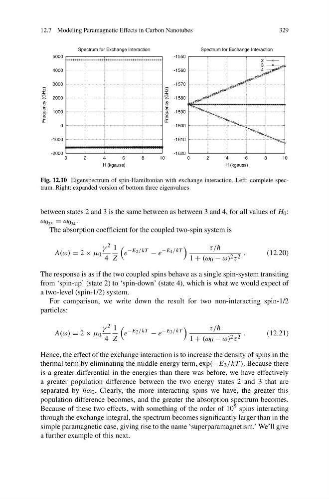
Fig. 12.10 Eigenspectrum of spin-Hamiltonian with exchange interaction. Left: complete spectrum. Right: expanded version of bottom three eigenvalues
between states 2 and 3 is the same between as between 3 and 4, for all values of H 0 :
ω 0 23 = ω 0 34 .
The absorption coefficient for the coupled two-spin system is
A(ω) = 2 × μ 0
γ 2
4
1
Z
e
−E 2 /kT
− e
−E 4 /kT
τ/ ¯
h
1 + (ω 0 − ω) 2 τ 2 .
(12.20)
The response is as if the two coupled spins behave as a single spin-system transiting
from ‘spin-up’ (state 2) to ‘spin-down’ (state 4), which is what we would expect of
a two-level (spin-1/2) system.
For comparison, we write down the result for two non-interacting spin-1/2
particles:
A(ω) = 2 × μ 0
γ 2
4
1
Z
e
−E 2 /kT
− e
−E 3 /kT
τ/ ¯
h
1 + (ω 0 − ω) 2 τ 2 .
(12.21)
Hence, the effect of the exchange interaction is to increase the density of spins in the
thermal term by eliminating the middle energy term, exp(−E 3 /kT ). Because there
is a greater differential in the energies than there was before, we have effectively
a greater population difference between the two energy states 2 and 3 that are
separated by ¯
hω 0 . Clearly, the more interacting spins we have, the greater this
population difference becomes, and the greater the absorption spectrum becomes.
Because of these two effects, with something of the order of 10 5 spins interacting
through the exchange integral, the spectrum becomes significantly larger than in the
simple paramagnetic case, giving rise to the name ‘superparamagnetism.’ We’ll give
a further example of this next.
329
-2000
-1000
0
1000
2000
3000
4000
5000
0
2
4
6
8
10
Frequency (GHz)
H (kgauss)
Spectrum for Exchange Interaction
-1620
-1610
-1600
-1590
-1580
-1570
-1560
-1550
0
2
4
6
8
10
Frequency (GHz)
H (kgauss)
Spectrum for Exchange Interaction
2
3
4
Fig. 12.10 Eigenspectrum of spin-Hamiltonian with exchange interaction. Left: complete spectrum. Right: expanded version of bottom three eigenvalues
between states 2 and 3 is the same between as between 3 and 4, for all values of H 0 :
ω 0 23 = ω 0 34 .
The absorption coefficient for the coupled two-spin system is
A(ω) = 2 × μ 0
γ 2
4
1
Z
e
−E 2 /kT
− e
−E 4 /kT
τ/ ¯
h
1 + (ω 0 − ω) 2 τ 2 .
(12.20)
The response is as if the two coupled spins behave as a single spin-system transiting
from ‘spin-up’ (state 2) to ‘spin-down’ (state 4), which is what we would expect of
a two-level (spin-1/2) system.
For comparison, we write down the result for two non-interacting spin-1/2
particles:
A(ω) = 2 × μ 0
γ 2
4
1
Z
e
−E 2 /kT
− e
−E 3 /kT
τ/ ¯
h
1 + (ω 0 − ω) 2 τ 2 .
(12.21)
Hence, the effect of the exchange interaction is to increase the density of spins in the
thermal term by eliminating the middle energy term, exp(−E 3 /kT ). Because there
is a greater differential in the energies than there was before, we have effectively
a greater population difference between the two energy states 2 and 3 that are
separated by ¯
hω 0 . Clearly, the more interacting spins we have, the greater this
population difference becomes, and the greater the absorption spectrum becomes.
Because of these two effects, with something of the order of 10 5 spins interacting
through the exchange integral, the spectrum becomes significantly larger than in the
simple paramagnetic case, giving rise to the name ‘superparamagnetism.’ We’ll give
a further example of this next.