

2.1 The Electromagnetic Model Equations
21
k
(k+1)
(k+2)
X
l
(l+1)
Y
m
( m + 1 )
Z
δ
δ
δ
δ
δ
δ
δ
x
x
x
y
y
z
z
1
1
1
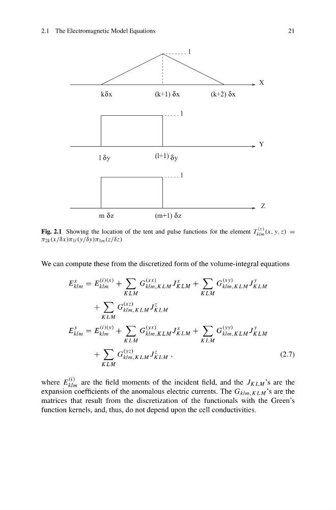
Fig. 2.1 Showing the location of the tent and pulse functions for the element T
(x)
klm (x, y, z) =
π 2k (x/δx)π 1l (y/δy)π 1m (z/δz)
We can compute these from the discretized form of the volume-integral equations
E
x
klm = E
(i)(x)
klm +
KLM
G
(xx)
klm,KLM J
x
KLM +
KLM
G
(xy)
klm,KLM J
y
KLM
+
KLM
G
(xz)
klm,KLM J
z
KLM
E
y
klm = E
(i)(y)
klm +
KLM
G
(yx)
klm,KLM J
x
KLM +
KLM
G
(yy)
klm,KLM J
y
KLM
+
KLM
G
(yz)
klm,KLM J
z
KLM ,
(2.7)
where E
(i)
klm are the field moments of the incident field, and the J KLM ’s are the
expansion coefficients of the anomalous electric currents. The G klm,KLM ’s are the
matrices that result from the discretization of the functionals with the Green’s
function kernels, and, thus, do not depend upon the cell conductivities.
21
k
(k+1)
(k+2)
X
l
(l+1)
Y
m
( m + 1 )
Z
δ
δ
δ
δ
δ
δ
δ
x
x
x
y
y
z
z
1
1
1
Fig. 2.1 Showing the location of the tent and pulse functions for the element T
(x)
klm (x, y, z) =
π 2k (x/δx)π 1l (y/δy)π 1m (z/δz)
We can compute these from the discretized form of the volume-integral equations
E
x
klm = E
(i)(x)
klm +
KLM
G
(xx)
klm,KLM J
x
KLM +
KLM
G
(xy)
klm,KLM J
y
KLM
+
KLM
G
(xz)
klm,KLM J
z
KLM
E
y
klm = E
(i)(y)
klm +
KLM
G
(yx)
klm,KLM J
x
KLM +
KLM
G
(yy)
klm,KLM J
y
KLM
+
KLM
G
(yz)
klm,KLM J
z
KLM ,
(2.7)
where E
(i)
klm are the field moments of the incident field, and the J KLM ’s are the
expansion coefficients of the anomalous electric currents. The G klm,KLM ’s are the
matrices that result from the discretization of the functionals with the Green’s
function kernels, and, thus, do not depend upon the cell conductivities.