

20
2 Voxel-Based Inversion Via Set-Theoretic Estimation
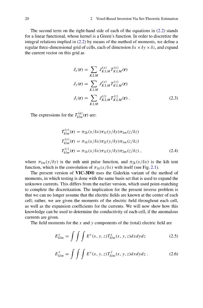
The second term on the right-hand side of each of the equations in (2.2) stands
for a linear functional, whose kernel is a Green’s function. In order to discretize the
integral relations implied in (2.2) by means of the method of moments, we define a
regular three-dimensional grid of cells, each of dimension δx × δy × δz, and expand
the current vector on this grid as
J x (r) =
KLM
J
(x)
KLM T
(x)
KLM (r)
J y (r) =
KLM
J
(y)
KLM T
(y)
KLM (r)
J z (r) =
KLM
J
(z)
KLM T
(z)
KLM (r) .
(2.3)
The expressions for the T
(q)
klm (r) are:
T
(x)
klm (r) = π 2k (x/δx)π 1l (y/δy)π 1m (z/δz)
T
(y)
klm (r) = π 1k (x/δx)π 2l (y/δy)π 1m (z/δz)
T
(z)
klm (r) = π 1k (x/δx)π 1l (y/δy)π 2m (z/δz) ,
(2.4)
where π 1m (y/δy) is the mth unit pulse function, and π 2k (x/δx) is the kth tent
function, which is the convolution of π 1k (x/δx) with itself (see Fig. 2.1).
The present version of VIC-3D® uses the Galerkin variant of the method of
moments, in which testing is done with the same basis set that is used to expand the
unknown currents. This differs from the earlier version, which used point-matching
to complete the discretization. The implication for the present inverse problem is
that we can no longer assume that the electric fields are known at the center of each
cell; rather, we are given the moments of the electric field throughout each cell,
as well as the expansion coefficients for the currents. We will now show how this
knowledge can be used to determine the conductivity of each cell, if the anomalous
currents are given.
The field moments for the x and y components of the (total) electric field are
E
x
klm =
E
x (x, y, z)T
x
klm (x, y, z)dxdydz
(2.5)
E
y
klm =
E
y (x, y, z)T
y
klm (x, y, z)dxdydz .
(2.6)
2 Voxel-Based Inversion Via Set-Theoretic Estimation
The second term on the right-hand side of each of the equations in (2.2) stands
for a linear functional, whose kernel is a Green’s function. In order to discretize the
integral relations implied in (2.2) by means of the method of moments, we define a
regular three-dimensional grid of cells, each of dimension δx × δy × δz, and expand
the current vector on this grid as
J x (r) =
KLM
J
(x)
KLM T
(x)
KLM (r)
J y (r) =
KLM
J
(y)
KLM T
(y)
KLM (r)
J z (r) =
KLM
J
(z)
KLM T
(z)
KLM (r) .
(2.3)
The expressions for the T
(q)
klm (r) are:
T
(x)
klm (r) = π 2k (x/δx)π 1l (y/δy)π 1m (z/δz)
T
(y)
klm (r) = π 1k (x/δx)π 2l (y/δy)π 1m (z/δz)
T
(z)
klm (r) = π 1k (x/δx)π 1l (y/δy)π 2m (z/δz) ,
(2.4)
where π 1m (y/δy) is the mth unit pulse function, and π 2k (x/δx) is the kth tent
function, which is the convolution of π 1k (x/δx) with itself (see Fig. 2.1).
The present version of VIC-3D® uses the Galerkin variant of the method of
moments, in which testing is done with the same basis set that is used to expand the
unknown currents. This differs from the earlier version, which used point-matching
to complete the discretization. The implication for the present inverse problem is
that we can no longer assume that the electric fields are known at the center of each
cell; rather, we are given the moments of the electric field throughout each cell,
as well as the expansion coefficients for the currents. We will now show how this
knowledge can be used to determine the conductivity of each cell, if the anomalous
currents are given.
The field moments for the x and y components of the (total) electric field are
E
x
klm =
E
x (x, y, z)T
x
klm (x, y, z)dxdydz
(2.5)
E
y
klm =
E
y (x, y, z)T
y
klm (x, y, z)dxdydz .
(2.6)