

292
11 Spintronics
S
(1)
x =
1
2
⎡
⎢
⎢
⎣
0 0 1 0
0 0 0 1
1 0 0 0
0 1 0 0
⎤
⎥
⎥
⎦ S
(1)
y =
1
2
⎡
⎢
⎢
⎣
0 0 −j 0
0 0 0 −j
j 0 0 0
0 j 0 0
⎤
⎥
⎥
⎦ S
(1)
z =
1
2
⎡
⎢
⎢
⎣
1 0 0 0
0 1 0 0
0 0 −1 0
0 0 0 −1
⎤
⎥
⎥
⎦
S
(2)
x =
1
2
⎡
⎢
⎢
⎣
0 1 0 0
1 0 0 0
0 0 0 1
0 0 1 0
⎤
⎥
⎥
⎦ S
(2)
y =
1
2
⎡
⎢
⎢
⎣
0 −j 0 0
j 0 0 0
0 0 0 −j
0 0 j 0
⎤
⎥
⎥
⎦ S
(2)
z =
1
2
⎡
⎢
⎢
⎣
1 0 0 0
0 −1 0 0
0 0 1 0
0 0 0 −1
⎤
⎥
⎥
⎦
(11.16)
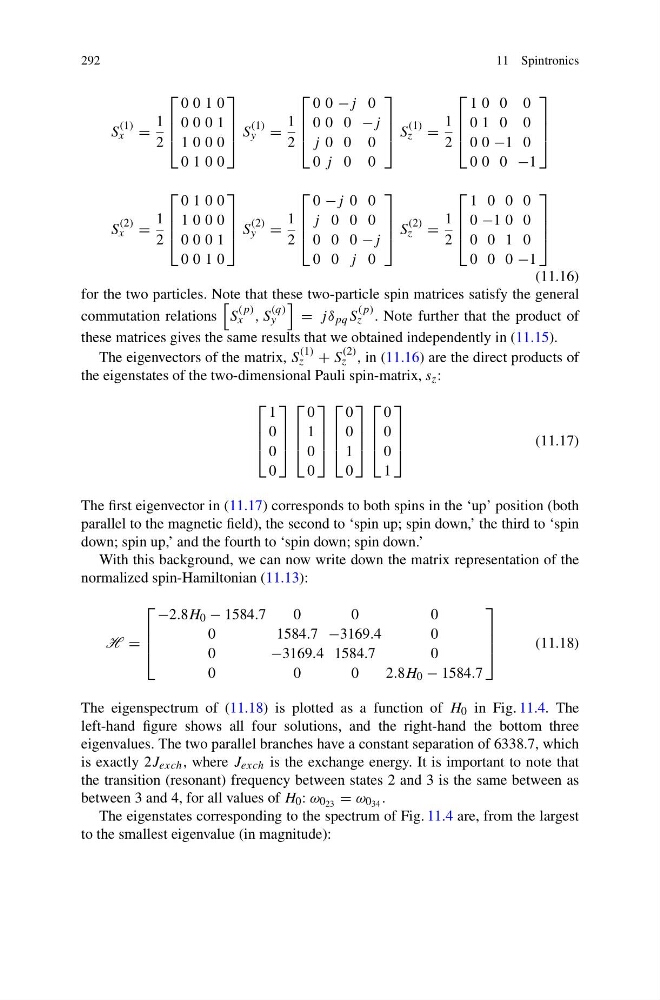
for the two particles. Note that these two-particle spin matrices satisfy the general
commutation relations
S
(p)
x , S
(q)
y
= jδ pq S
(p)
z . Note further that the product of
these matrices gives the same results that we obtained independently in (11.15).
The eigenvectors of the matrix, S
(1)
z + S
(2)
z , in (11.16) are the direct products of
the eigenstates of the two-dimensional Pauli spin-matrix, s z :
⎡
⎢
⎢
⎣
1
0
0
0
⎤
⎥
⎥
⎦
⎡
⎢
⎢
⎣
0
1
0
0
⎤
⎥
⎥
⎦
⎡
⎢
⎢
⎣
0
0
1
0
⎤
⎥
⎥
⎦
⎡
⎢
⎢
⎣
0
0
0
1
⎤
⎥
⎥
⎦
(11.17)
The first eigenvector in (11.17) corresponds to both spins in the ‘up’ position (both
parallel to the magnetic field), the second to ‘spin up; spin down,’ the third to ‘spin
down; spin up,’ and the fourth to ‘spin down; spin down.’
With this background, we can now write down the matrix representation of the
normalized spin-Hamiltonian (11.13):
H =
⎡
⎢
⎢
⎣
−2.8H 0 − 1584.7
0
0
0
0
1584.7 −3169.4
0
0
−3169.4 1584.7
0
0
0
0
2 .8H 0 − 1584.7
⎤
⎥
⎥
⎦
(11.18)
The eigenspectrum of (11.18) is plotted as a function of H 0 in Fig. 11.4. The
left-hand figure shows all four solutions, and the right-hand the bottom three
eigenvalues. The two parallel branches have a constant separation of 6338.7, which
is exactly 2J exch , where J exch is the exchange energy. It is important to note that
the transition (resonant) frequency between states 2 and 3 is the same between as
between 3 and 4, for all values of H 0 : ω 0 23 = ω 0 34 .
The eigenstates corresponding to the spectrum of Fig. 11.4 are, from the largest
to the smallest eigenvalue (in magnitude):
11 Spintronics
S
(1)
x =
1
2
⎡
⎢
⎢
⎣
0 0 1 0
0 0 0 1
1 0 0 0
0 1 0 0
⎤
⎥
⎥
⎦ S
(1)
y =
1
2
⎡
⎢
⎢
⎣
0 0 −j 0
0 0 0 −j
j 0 0 0
0 j 0 0
⎤
⎥
⎥
⎦ S
(1)
z =
1
2
⎡
⎢
⎢
⎣
1 0 0 0
0 1 0 0
0 0 −1 0
0 0 0 −1
⎤
⎥
⎥
⎦
S
(2)
x =
1
2
⎡
⎢
⎢
⎣
0 1 0 0
1 0 0 0
0 0 0 1
0 0 1 0
⎤
⎥
⎥
⎦ S
(2)
y =
1
2
⎡
⎢
⎢
⎣
0 −j 0 0
j 0 0 0
0 0 0 −j
0 0 j 0
⎤
⎥
⎥
⎦ S
(2)
z =
1
2
⎡
⎢
⎢
⎣
1 0 0 0
0 −1 0 0
0 0 1 0
0 0 0 −1
⎤
⎥
⎥
⎦
(11.16)
for the two particles. Note that these two-particle spin matrices satisfy the general
commutation relations
S
(p)
x , S
(q)
y
= jδ pq S
(p)
z . Note further that the product of
these matrices gives the same results that we obtained independently in (11.15).
The eigenvectors of the matrix, S
(1)
z + S
(2)
z , in (11.16) are the direct products of
the eigenstates of the two-dimensional Pauli spin-matrix, s z :
⎡
⎢
⎢
⎣
1
0
0
0
⎤
⎥
⎥
⎦
⎡
⎢
⎢
⎣
0
1
0
0
⎤
⎥
⎥
⎦
⎡
⎢
⎢
⎣
0
0
1
0
⎤
⎥
⎥
⎦
⎡
⎢
⎢
⎣
0
0
0
1
⎤
⎥
⎥
⎦
(11.17)
The first eigenvector in (11.17) corresponds to both spins in the ‘up’ position (both
parallel to the magnetic field), the second to ‘spin up; spin down,’ the third to ‘spin
down; spin up,’ and the fourth to ‘spin down; spin down.’
With this background, we can now write down the matrix representation of the
normalized spin-Hamiltonian (11.13):
H =
⎡
⎢
⎢
⎣
−2.8H 0 − 1584.7
0
0
0
0
1584.7 −3169.4
0
0
−3169.4 1584.7
0
0
0
0
2 .8H 0 − 1584.7
⎤
⎥
⎥
⎦
(11.18)
The eigenspectrum of (11.18) is plotted as a function of H 0 in Fig. 11.4. The
left-hand figure shows all four solutions, and the right-hand the bottom three
eigenvalues. The two parallel branches have a constant separation of 6338.7, which
is exactly 2J exch , where J exch is the exchange energy. It is important to note that
the transition (resonant) frequency between states 2 and 3 is the same between as
between 3 and 4, for all values of H 0 : ω 0 23 = ω 0 34 .
The eigenstates corresponding to the spectrum of Fig. 11.4 are, from the largest
to the smallest eigenvalue (in magnitude):