

11.2 Paramagnetic Spin Dynamics and the Spin Hamiltonian
289
approximation to the effective spin-Hamiltonian we may discard any terms that
represent the crystalline field. We must, however, include the spin-spin interaction
between the unpaired electrons and the nucleus because these electrons are relatively
close to the nucleus. Thus, we use the following spin-Hamiltonian
H 0 = gβH 0 · S + AI · S ,
(11.11)
where g = 5.91, β = 0.0014 GHz/gauss, A = 3.924 GHz, S is the electron spin
operator, with effective spin 1/2, and I is the nuclear spin operator with spin 7/2.
Because we are dealing with a system of two particles (electron plus nucleus)
we cannot simply form matrix products in order to evaluate H 0 , but must use the
direct product of the appropriate Pauli spin matrices of I and S. Because there are
two possible electron spin-states (“spin up” and “spin down” relative to, say, the
axis of H 0 ) and 2 × 7/2 + 1 = 8 possible spin states of the nucleus, we have
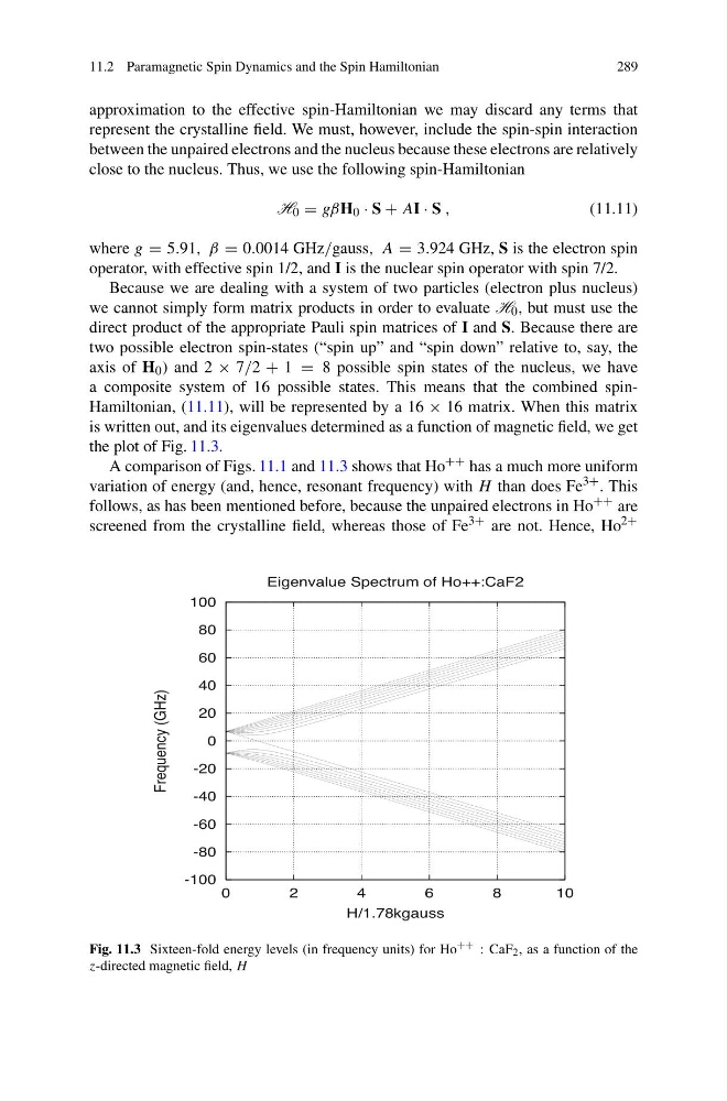
a composite system of 16 possible states. This means that the combined spinHamiltonian, (11.11), will be represented by a 16 × 16 matrix. When this matrix
is written out, and its eigenvalues determined as a function of magnetic field, we get
the plot of Fig. 11.3.
A comparison of Figs. 11.1 and 11.3 shows that Ho
++ has a much more uniform
variation of energy (and, hence, resonant frequency) with H than does Fe
3+ . This
follows, as has been mentioned before, because the unpaired electrons in Ho
++ are
screened from the crystalline field, whereas those of Fe
3+ are not. Hence, Ho
2+
-100
-80
-60
-40
-20
0
20
40
60
80
100
0
2
4
6
8
10
Frequency (GHz)
H/1.78kgauss
Eigenvalue Spectrum of Ho++:CaF2
Fig. 11.3 Sixteen-fold energy levels (in frequency units) for Ho
++ : CaF 2 , as a function of the
z-directed magnetic field, H
289
approximation to the effective spin-Hamiltonian we may discard any terms that
represent the crystalline field. We must, however, include the spin-spin interaction
between the unpaired electrons and the nucleus because these electrons are relatively
close to the nucleus. Thus, we use the following spin-Hamiltonian
H 0 = gβH 0 · S + AI · S ,
(11.11)
where g = 5.91, β = 0.0014 GHz/gauss, A = 3.924 GHz, S is the electron spin
operator, with effective spin 1/2, and I is the nuclear spin operator with spin 7/2.
Because we are dealing with a system of two particles (electron plus nucleus)
we cannot simply form matrix products in order to evaluate H 0 , but must use the
direct product of the appropriate Pauli spin matrices of I and S. Because there are
two possible electron spin-states (“spin up” and “spin down” relative to, say, the
axis of H 0 ) and 2 × 7/2 + 1 = 8 possible spin states of the nucleus, we have
a composite system of 16 possible states. This means that the combined spinHamiltonian, (11.11), will be represented by a 16 × 16 matrix. When this matrix
is written out, and its eigenvalues determined as a function of magnetic field, we get
the plot of Fig. 11.3.
A comparison of Figs. 11.1 and 11.3 shows that Ho
++ has a much more uniform
variation of energy (and, hence, resonant frequency) with H than does Fe
3+ . This
follows, as has been mentioned before, because the unpaired electrons in Ho
++ are
screened from the crystalline field, whereas those of Fe
3+ are not. Hence, Ho
2+
-100
-80
-60
-40
-20
0
20
40
60
80
100
0
2
4
6
8
10
Frequency (GHz)
H/1.78kgauss
Eigenvalue Spectrum of Ho++:CaF2
Fig. 11.3 Sixteen-fold energy levels (in frequency units) for Ho
++ : CaF 2 , as a function of the
z-directed magnetic field, H