

218
9 High-Dimension Model Representation via Sparse GridTechniques
Table 9.1 Four-dimensional
vectors satisfying |l| ∞ ≤ 1.
The last column gives the
number of nodes associated
with each vector
0
0
0
0
16
1
0
0
0
8
0
1
0
0
8
0
0
1
0
8
0
0
0
1
8
1
1
0
0
4
1
0
1
0
4
1
0
0
1
4
0
1
0
1
4
0
0
1
1
4
0
1
1
0
4
1
1
0
1
2
1
0
1
1
2
0
1
1
1
2
1
1
1
0
2
1
1
1
1
1
Total
81
Table 9.2 Four-dimensional
vectors satisfying |l| 1 ≤ 1.
The last column gives the
number of nodes associated
with each vector
0
0
0
0
16
1
0
0
0
8
0
1
0
0
8
0
0
1
0
8
0
0
0
1
8
Total
48
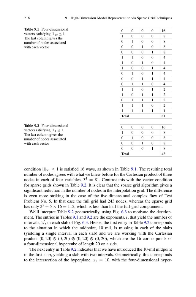
condition |l| ∞ ≤ 1 is satisfied 16 ways, as shown in Table 9.1. The resulting total
number of nodes agrees with what we knew before for the Cartesian product of three
nodes in each of four variables, 3 4 = 81. Contrast this with the vector condition
for sparse grids shown in Table 9.2. It is clear that the sparse grid algorithm gives a
significant reduction in the number of nodes in the interpolation grid. The difference
is even more striking in the case of the five-dimensional complex flaw of Test
Problem No. 5. In that case the full grid had 243 nodes, whereas the sparse grid
has only 2 5 + 5 × 16 = 112, which is less than half the full-grid complement.
We’ll interpret Table 9.2 geometrically, using Fig. 6.3 to motivate the development. The entries in Tables 9.1 and 9.2 are the exponents, l, that yield the number of
intervals, 2 l , in each slab of Fig. 6.3. Hence, the first entry in Table 9.2 corresponds
to the situation in which the midpoint, 10 mil, is missing in each of the slabs
(yielding a single interval in each slab) and we are working with the Cartesian
product (0, 20) ⊗ (0, 20) ⊗ (0, 20) ⊗ (0, 20), which are the 16 corner points of
a four-dimensional hypercube of length 20 on a side.
The next entry in Table 9.2 indicates that we have introduced the 10-mil midpoint
in the first slab, yielding a slab with two intervals. Geometrically, this corresponds
to the intersection of the hyperplane, x 1 = 10, with the four-dimensional hyper-
9 High-Dimension Model Representation via Sparse GridTechniques
Table 9.1 Four-dimensional
vectors satisfying |l| ∞ ≤ 1.
The last column gives the
number of nodes associated
with each vector
0
0
0
0
16
1
0
0
0
8
0
1
0
0
8
0
0
1
0
8
0
0
0
1
8
1
1
0
0
4
1
0
1
0
4
1
0
0
1
4
0
1
0
1
4
0
0
1
1
4
0
1
1
0
4
1
1
0
1
2
1
0
1
1
2
0
1
1
1
2
1
1
1
0
2
1
1
1
1
1
Total
81
Table 9.2 Four-dimensional
vectors satisfying |l| 1 ≤ 1.
The last column gives the
number of nodes associated
with each vector
0
0
0
0
16
1
0
0
0
8
0
1
0
0
8
0
0
1
0
8
0
0
0
1
8
Total
48
condition |l| ∞ ≤ 1 is satisfied 16 ways, as shown in Table 9.1. The resulting total
number of nodes agrees with what we knew before for the Cartesian product of three
nodes in each of four variables, 3 4 = 81. Contrast this with the vector condition
for sparse grids shown in Table 9.2. It is clear that the sparse grid algorithm gives a
significant reduction in the number of nodes in the interpolation grid. The difference
is even more striking in the case of the five-dimensional complex flaw of Test
Problem No. 5. In that case the full grid had 243 nodes, whereas the sparse grid
has only 2 5 + 5 × 16 = 112, which is less than half the full-grid complement.
We’ll interpret Table 9.2 geometrically, using Fig. 6.3 to motivate the development. The entries in Tables 9.1 and 9.2 are the exponents, l, that yield the number of
intervals, 2 l , in each slab of Fig. 6.3. Hence, the first entry in Table 9.2 corresponds
to the situation in which the midpoint, 10 mil, is missing in each of the slabs
(yielding a single interval in each slab) and we are working with the Cartesian
product (0, 20) ⊗ (0, 20) ⊗ (0, 20) ⊗ (0, 20), which are the 16 corner points of
a four-dimensional hypercube of length 20 on a side.
The next entry in Table 9.2 indicates that we have introduced the 10-mil midpoint
in the first slab, yielding a slab with two intervals. Geometrically, this corresponds
to the intersection of the hyperplane, x 1 = 10, with the four-dimensional hyper-