

8.6 Results for the Anisotropic Double-Exponential Model
211
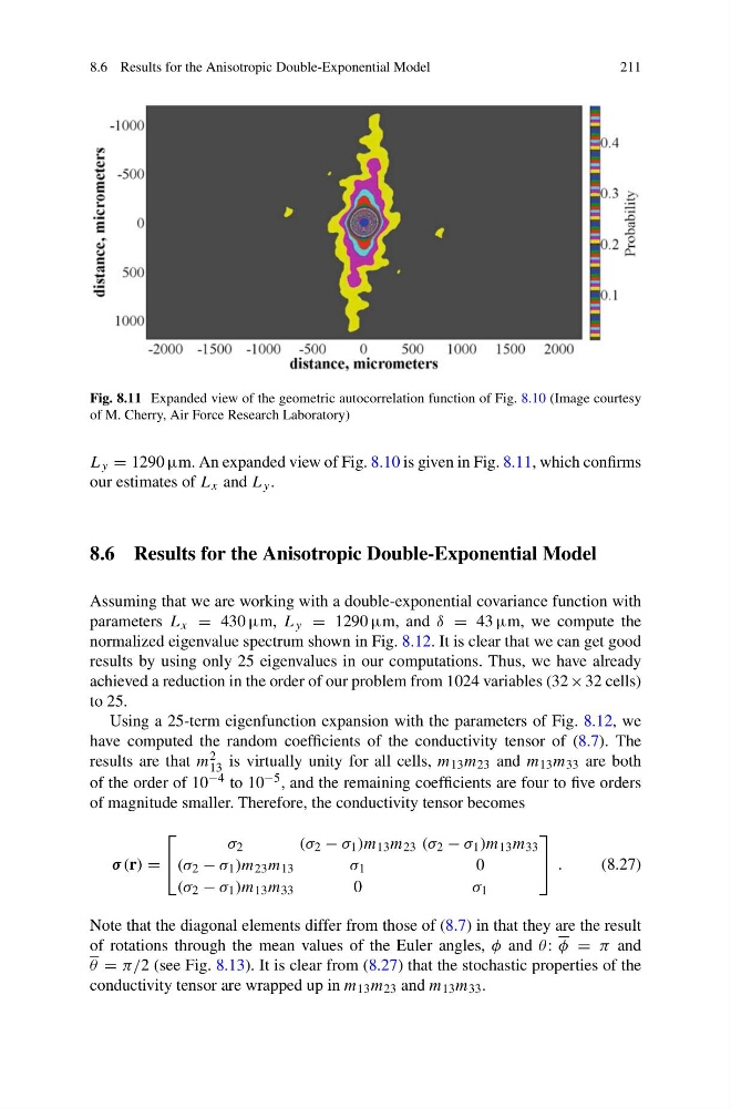
Fig. 8.11 Expanded view of the geometric autocorrelation function of Fig. 8.10 (Image courtesy
of M. Cherry, Air Force Research Laboratory)
L y = 1290 µm. An expanded view of Fig. 8.10 is given in Fig. 8.11, which confirms
our estimates of L x and L y .
8.6 Results for the Anisotropic Double-Exponential Model
Assuming that we are working with a double-exponential covariance function with
parameters L x = 430 µm, L y = 1290 µm, and δ = 43 µm, we compute the
normalized eigenvalue spectrum shown in Fig. 8.12. It is clear that we can get good
results by using only 25 eigenvalues in our computations. Thus, we have already
achieved a reduction in the order of our problem from 1024 variables (32 × 32 cells)
to 25.
Using a 25-term eigenfunction expansion with the parameters of Fig. 8.12, we
have computed the random coefficients of the conductivity tensor of (8.7). The
results are that m 2
13 is virtually unity for all cells, m 13 m 23 and m 13 m 33 are both
of the order of 10 −4 to 10 −5 , and the remaining coefficients are four to five orders
of magnitude smaller. Therefore, the conductivity tensor becomes
σ (r) =
⎡
⎣
σ 2
(σ 2 − σ 1 )m 13 m 23 (σ 2 − σ 1 )m 13 m 33
(σ 2 − σ 1 )m 23 m 13
σ 1
0
(σ 2 − σ 1 )m 13 m 33
0
σ 1
⎤
⎦ .
(8.27)
Note that the diagonal elements differ from those of (8.7) in that they are the result
of rotations through the mean values of the Euler angles, φ and θ : φ = π and
θ = π/2 (see Fig. 8.13). It is clear from (8.27) that the stochastic properties of the
conductivity tensor are wrapped up in m 13 m 23 and m 13 m 33 .
211
Fig. 8.11 Expanded view of the geometric autocorrelation function of Fig. 8.10 (Image courtesy
of M. Cherry, Air Force Research Laboratory)
L y = 1290 µm. An expanded view of Fig. 8.10 is given in Fig. 8.11, which confirms
our estimates of L x and L y .
8.6 Results for the Anisotropic Double-Exponential Model
Assuming that we are working with a double-exponential covariance function with
parameters L x = 430 µm, L y = 1290 µm, and δ = 43 µm, we compute the
normalized eigenvalue spectrum shown in Fig. 8.12. It is clear that we can get good
results by using only 25 eigenvalues in our computations. Thus, we have already
achieved a reduction in the order of our problem from 1024 variables (32 × 32 cells)
to 25.
Using a 25-term eigenfunction expansion with the parameters of Fig. 8.12, we
have computed the random coefficients of the conductivity tensor of (8.7). The
results are that m 2
13 is virtually unity for all cells, m 13 m 23 and m 13 m 33 are both
of the order of 10 −4 to 10 −5 , and the remaining coefficients are four to five orders
of magnitude smaller. Therefore, the conductivity tensor becomes
σ (r) =
⎡
⎣
σ 2
(σ 2 − σ 1 )m 13 m 23 (σ 2 − σ 1 )m 13 m 33
(σ 2 − σ 1 )m 23 m 13
σ 1
0
(σ 2 − σ 1 )m 13 m 33
0
σ 1
⎤
⎦ .
(8.27)
Note that the diagonal elements differ from those of (8.7) in that they are the result
of rotations through the mean values of the Euler angles, φ and θ : φ = π and
θ = π/2 (see Fig. 8.13). It is clear from (8.27) that the stochastic properties of the
conductivity tensor are wrapped up in m 13 m 23 and m 13 m 33 .