

206
8 A Model for Microstructure Characterization
0
0.1
0.2
0.3
0.4
0.5
0.6
0.7
0.8
0.9
1
0
10
20
30
40
50
60
70
80
90 100
Normalized eigenvalue spectra for two 2D-covariances
Gaussian
Double-Exponential
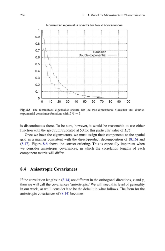
Fig. 8.5 The normalized eigenvalue spectra for the two-dimensional Gaussian and doubleexponential covariance functions with L/δ = 5
is discontinuous there. To be sure, however, it would be reasonable to use either
function with the spectrum truncated at 50 for this particular value of L/δ.
Once we have the eigenvectors, we must assign their components to the spatial
grid in a manner consistent with the direct-product decomposition of (8.16) and
(8.17). Figure 8.6 shows the correct ordering. This is especially important when
we consider anisotropic covariances, in which the correlation lengths of each
component matrix will differ.
8.4 Anisotropic Covariances
If the correlation lengths in (8.14) are different in the orthogonal directions, x and y,
then we will call the covariances ‘anisotropic.’ We will need this level of generality
in our work, so we’ll consider it to be the default in what follows. The form for the
anisotropic covariances of (8.14) becomes:
8 A Model for Microstructure Characterization
0
0.1
0.2
0.3
0.4
0.5
0.6
0.7
0.8
0.9
1
0
10
20
30
40
50
60
70
80
90 100
Normalized eigenvalue spectra for two 2D-covariances
Gaussian
Double-Exponential
Fig. 8.5 The normalized eigenvalue spectra for the two-dimensional Gaussian and doubleexponential covariance functions with L/δ = 5
is discontinuous there. To be sure, however, it would be reasonable to use either
function with the spectrum truncated at 50 for this particular value of L/δ.
Once we have the eigenvectors, we must assign their components to the spatial
grid in a manner consistent with the direct-product decomposition of (8.16) and
(8.17). Figure 8.6 shows the correct ordering. This is especially important when
we consider anisotropic covariances, in which the correlation lengths of each
component matrix will differ.
8.4 Anisotropic Covariances
If the correlation lengths in (8.14) are different in the orthogonal directions, x and y,
then we will call the covariances ‘anisotropic.’ We will need this level of generality
in our work, so we’ll consider it to be the default in what follows. The form for the
anisotropic covariances of (8.14) becomes: