

8.3 The Karhunen-Loève Model
205
erf z =
2
√
π
∞
n=0
(−1) n z 2n+1
n!(2n + 1)
,
(8.21)
into (8.20):
G
(x)
mm = sL
2
∞
n=0
(−1) n
n!(2n + 1)
(m −m+1)δ/L
(m −m)δ/L
v
2n+1 − (v − δ/L)
2n+1
dv
= sL
2
∞
n=0
(−1) n
n!(2n + 1)
v 2n+2
2n + 2
−
(v − δ/L) 2n+2
2n + 2
(m −m+1)δ/L
(m −m)δ/L
= sL
2
∞
n=0
(−1) n
n!(2n + 1)(2n + 2)
[(m
− m + 1)(δ/L)]
2n+2 − 2[(m
− m)(δ/L)]
2n+2
+[(m
− m − 1)(δ/L)]
2n+2
(8.22)
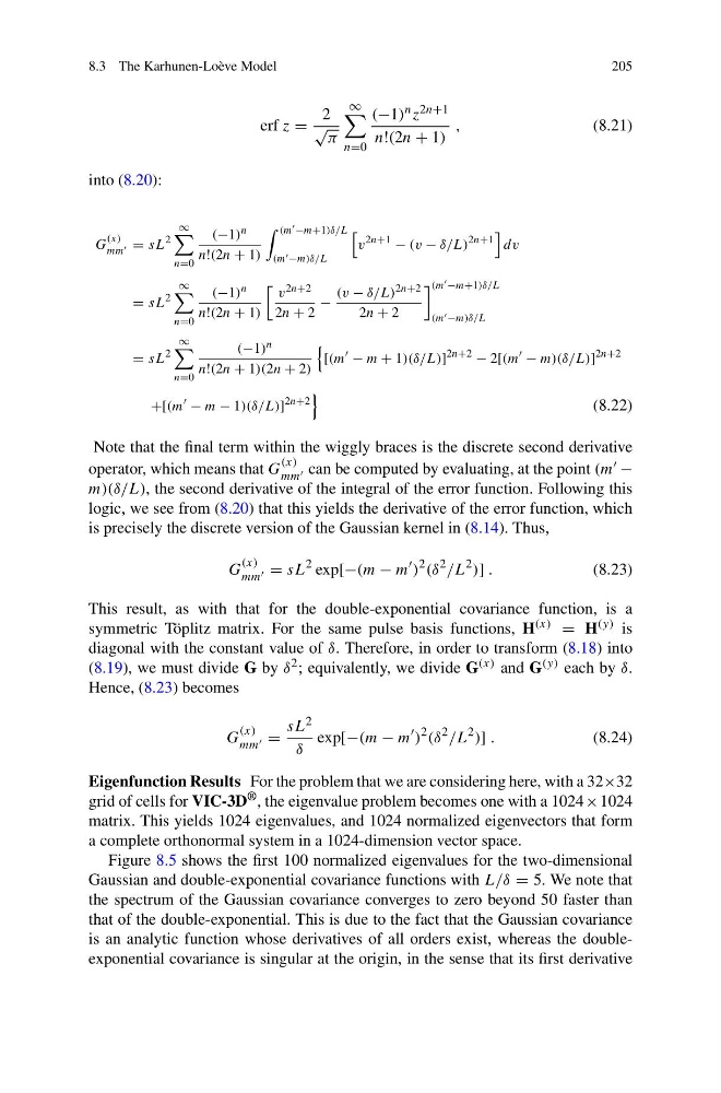
Note that the final term within the wiggly braces is the discrete second derivative
operator, which means that G
(x)
mm can be computed by evaluating, at the point (m −
m)(δ/L), the second derivative of the integral of the error function. Following this
logic, we see from (8.20) that this yields the derivative of the error function, which
is precisely the discrete version of the Gaussian kernel in (8.14). Thus,
G
(x)
mm = sL
2 exp[−(m − m
)
2 (δ
2 /L
2 )] .
(8.23)
This result, as with that for the double-exponential covariance function, is a
symmetric Töplitz matrix. For the same pulse basis functions, H (x) = H (y) is
diagonal with the constant value of δ. Therefore, in order to transform (8.18) into
(8.19), we must divide G by δ 2 ; equivalently, we divide G (x) and G (y) each by δ.
Hence, (8.23) becomes
G
(x)
mm =
sL 2
δ
exp[−(m − m
)
2 (δ
2 /L
2 )] .
(8.24)
Eigenfunction Results For the problem that we are considering here, with a 32×32
grid of cells for VIC-3D ® , the eigenvalue problem becomes one with a 1024 × 1024
matrix. This yields 1024 eigenvalues, and 1024 normalized eigenvectors that form
a complete orthonormal system in a 1024-dimension vector space.
Figure 8.5 shows the first 100 normalized eigenvalues for the two-dimensional
Gaussian and double-exponential covariance functions with L/δ = 5. We note that
the spectrum of the Gaussian covariance converges to zero beyond 50 faster than
that of the double-exponential. This is due to the fact that the Gaussian covariance
is an analytic function whose derivatives of all orders exist, whereas the doubleexponential covariance is singular at the origin, in the sense that its first derivative
205
erf z =
2
√
π
∞
n=0
(−1) n z 2n+1
n!(2n + 1)
,
(8.21)
into (8.20):
G
(x)
mm = sL
2
∞
n=0
(−1) n
n!(2n + 1)
(m −m+1)δ/L
(m −m)δ/L
v
2n+1 − (v − δ/L)
2n+1
dv
= sL
2
∞
n=0
(−1) n
n!(2n + 1)
v 2n+2
2n + 2
−
(v − δ/L) 2n+2
2n + 2
(m −m+1)δ/L
(m −m)δ/L
= sL
2
∞
n=0
(−1) n
n!(2n + 1)(2n + 2)
[(m
− m + 1)(δ/L)]
2n+2 − 2[(m
− m)(δ/L)]
2n+2
+[(m
− m − 1)(δ/L)]
2n+2
(8.22)
Note that the final term within the wiggly braces is the discrete second derivative
operator, which means that G
(x)
mm can be computed by evaluating, at the point (m −
m)(δ/L), the second derivative of the integral of the error function. Following this
logic, we see from (8.20) that this yields the derivative of the error function, which
is precisely the discrete version of the Gaussian kernel in (8.14). Thus,
G
(x)
mm = sL
2 exp[−(m − m
)
2 (δ
2 /L
2 )] .
(8.23)
This result, as with that for the double-exponential covariance function, is a
symmetric Töplitz matrix. For the same pulse basis functions, H (x) = H (y) is
diagonal with the constant value of δ. Therefore, in order to transform (8.18) into
(8.19), we must divide G by δ 2 ; equivalently, we divide G (x) and G (y) each by δ.
Hence, (8.23) becomes
G
(x)
mm =
sL 2
δ
exp[−(m − m
)
2 (δ
2 /L
2 )] .
(8.24)
Eigenfunction Results For the problem that we are considering here, with a 32×32
grid of cells for VIC-3D ® , the eigenvalue problem becomes one with a 1024 × 1024
matrix. This yields 1024 eigenvalues, and 1024 normalized eigenvectors that form
a complete orthonormal system in a 1024-dimension vector space.
Figure 8.5 shows the first 100 normalized eigenvalues for the two-dimensional
Gaussian and double-exponential covariance functions with L/δ = 5. We note that
the spectrum of the Gaussian covariance converges to zero beyond 50 faster than
that of the double-exponential. This is due to the fact that the Gaussian covariance
is an analytic function whose derivatives of all orders exist, whereas the doubleexponential covariance is singular at the origin, in the sense that its first derivative