

7.9 Two-Dimensional Functions
181
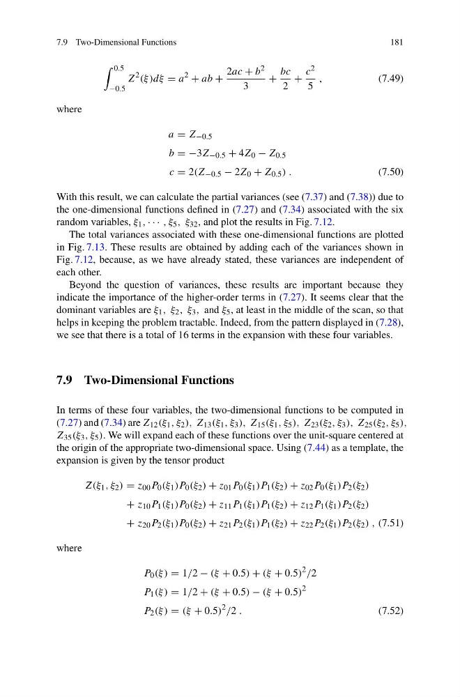
0.5
−0.5
Z
2 (ξ )dξ = a
2
+ ab +
2ac + b 2
3
+
bc
2
+
c 2
5
,
(7.49)
where
a = Z −0.5
b = −3Z −0.5 + 4Z 0 − Z 0.5
c = 2(Z −0.5 − 2Z 0 + Z 0.5 ) .
(7.50)
With this result, we can calculate the partial variances (see (7.37) and (7.38)) due to
the one-dimensional functions defined in (7.27) and (7.34) associated with the six
random variables, ξ 1 , · · · , ξ 5 , ξ 32 , and plot the results in Fig. 7.12.
The total variances associated with these one-dimensional functions are plotted
in Fig. 7.13. These results are obtained by adding each of the variances shown in
Fig. 7.12, because, as we have already stated, these variances are independent of
each other.
Beyond the question of variances, these results are important because they
indicate the importance of the higher-order terms in (7.27). It seems clear that the
dominant variables are ξ 1 , ξ 2 , ξ 3 , and ξ 5 , at least in the middle of the scan, so that
helps in keeping the problem tractable. Indeed, from the pattern displayed in (7.28),
we see that there is a total of 16 terms in the expansion with these four variables.
7.9 Two-Dimensional Functions
In terms of these four variables, the two-dimensional functions to be computed in
(7.27) and (7.34) are Z 12 (ξ 1 , ξ 2 ), Z 13 (ξ 1 , ξ 3 ), Z 15 (ξ 1 , ξ 5 ), Z 23 (ξ 2 , ξ 3 ), Z 25 (ξ 2 , ξ 5 ),
Z 35 (ξ 3 , ξ 5 ). We will expand each of these functions over the unit-square centered at
the origin of the appropriate two-dimensional space. Using (7.44) as a template, the
expansion is given by the tensor product
Z(ξ 1 , ξ 2 ) = z 00 P 0 (ξ 1 )P 0 (ξ 2 ) + z 01 P 0 (ξ 1 )P 1 (ξ 2 ) + z 02 P 0 (ξ 1 )P 2 (ξ 2 )
+ z 10 P 1 (ξ 1 )P 0 (ξ 2 ) + z 11 P 1 (ξ 1 )P 1 (ξ 2 ) + z 12 P 1 (ξ 1 )P 2 (ξ 2 )
+ z 20 P 2 (ξ 1 )P 0 (ξ 2 ) + z 21 P 2 (ξ 1 )P 1 (ξ 2 ) + z 22 P 2 (ξ 1 )P 2 (ξ 2 ) , (7.51)
where
P 0 (ξ ) = 1/2 − (ξ + 0.5) + (ξ + 0.5)
2 /2
P 1 (ξ ) = 1/2 + (ξ + 0.5) − (ξ + 0.5)
2
P 2 (ξ ) = (ξ + 0.5)
2 /2 .
(7.52)
181
0.5
−0.5
Z
2 (ξ )dξ = a
2
+ ab +
2ac + b 2
3
+
bc
2
+
c 2
5
,
(7.49)
where
a = Z −0.5
b = −3Z −0.5 + 4Z 0 − Z 0.5
c = 2(Z −0.5 − 2Z 0 + Z 0.5 ) .
(7.50)
With this result, we can calculate the partial variances (see (7.37) and (7.38)) due to
the one-dimensional functions defined in (7.27) and (7.34) associated with the six
random variables, ξ 1 , · · · , ξ 5 , ξ 32 , and plot the results in Fig. 7.12.
The total variances associated with these one-dimensional functions are plotted
in Fig. 7.13. These results are obtained by adding each of the variances shown in
Fig. 7.12, because, as we have already stated, these variances are independent of
each other.
Beyond the question of variances, these results are important because they
indicate the importance of the higher-order terms in (7.27). It seems clear that the
dominant variables are ξ 1 , ξ 2 , ξ 3 , and ξ 5 , at least in the middle of the scan, so that
helps in keeping the problem tractable. Indeed, from the pattern displayed in (7.28),
we see that there is a total of 16 terms in the expansion with these four variables.
7.9 Two-Dimensional Functions
In terms of these four variables, the two-dimensional functions to be computed in
(7.27) and (7.34) are Z 12 (ξ 1 , ξ 2 ), Z 13 (ξ 1 , ξ 3 ), Z 15 (ξ 1 , ξ 5 ), Z 23 (ξ 2 , ξ 3 ), Z 25 (ξ 2 , ξ 5 ),
Z 35 (ξ 3 , ξ 5 ). We will expand each of these functions over the unit-square centered at
the origin of the appropriate two-dimensional space. Using (7.44) as a template, the
expansion is given by the tensor product
Z(ξ 1 , ξ 2 ) = z 00 P 0 (ξ 1 )P 0 (ξ 2 ) + z 01 P 0 (ξ 1 )P 1 (ξ 2 ) + z 02 P 0 (ξ 1 )P 2 (ξ 2 )
+ z 10 P 1 (ξ 1 )P 0 (ξ 2 ) + z 11 P 1 (ξ 1 )P 1 (ξ 2 ) + z 12 P 1 (ξ 1 )P 2 (ξ 2 )
+ z 20 P 2 (ξ 1 )P 0 (ξ 2 ) + z 21 P 2 (ξ 1 )P 1 (ξ 2 ) + z 22 P 2 (ξ 1 )P 2 (ξ 2 ) , (7.51)
where
P 0 (ξ ) = 1/2 − (ξ + 0.5) + (ξ + 0.5)
2 /2
P 1 (ξ ) = 1/2 + (ξ + 0.5) − (ξ + 0.5)
2
P 2 (ξ ) = (ξ + 0.5)
2 /2 .
(7.52)