

7.8 Interpolation Theory Using Splines Based Upon Higher-Order. . .
179
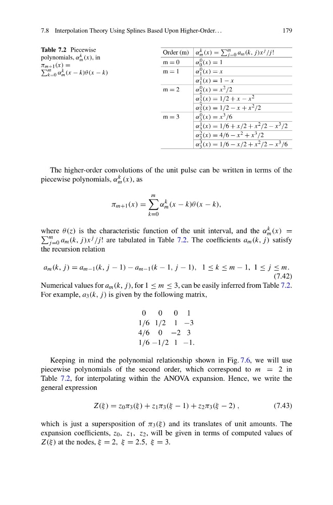
Table 7.2 Piecewise
polynomials, α k
m (x), in
π m+1 (x) =
m
k=0 α k
m (x − k)θ(x − k)
Order (m) α k
m (x) =
m
j =0 a m (k, j )x j /j !
m = 0
α 0
0 (x) = 1
m = 1
α 0
1 (x) = x
α 1
1 (x) = 1 − x
m = 2
α 0
2 (x) = x 2 /2
α 1
2 (x) = 1/2 + x − x 2
α 2
2 (x) = 1/2 − x + x 2 /2
m = 3
α 0
3 (x) = x 3 /6
α 1
3 (x) = 1/6 + x/2 + x 2 /2 − x 3 /2
α 2
3 (x) = 4/6 − x 2 + x 3 /2
α 3
3 (x) = 1/6 − x/2 + x 2 /2 − x 3 /6
The higher-order convolutions of the unit pulse can be written in terms of the
piecewise polynomials, α k
m (x), as
π m+1 (x) =
m
k=0
α
k
m (x − k)θ(x − k),
where θ(z) is the characteristic function of the unit interval, and the α k
m (x) =
m
j =0 a m (k, j )x j /j ! are tabulated in Table 7.2. The coefficients a m (k, j ) satisfy
the recursion relation
a m (k, j ) = a m−1 (k, j − 1) − a m−1 (k − 1, j − 1), 1 ≤ k ≤ m − 1, 1 ≤ j ≤ m.
(7.42)
Numerical values for a m (k, j ), for 1 ≤ m ≤ 3, can be easily inferred from Table 7.2.
For example, a 3 (k, j ) is given by the following matrix,
0
0
0 1
1/6 1/2 1 −3
4/6 0 −2 3
1/6 −1/2 1 −1.
Keeping in mind the polynomial relationship shown in Fig. 7.6, we will use
piecewise polynomials of the second order, which correspond to m = 2 in
Table 7.2, for interpolating within the ANOVA expansion. Hence, we write the
general expression
Z(ξ ) = z 0 π 3 (ξ ) + z 1 π 3 (ξ − 1) + z 2 π 3 (ξ − 2) ,
(7.43)
which is just a supersposition of π 3 (ξ ) and its translates of unit amounts. The
expansion coefficients, z 0 , z 1 , z 2 , will be given in terms of computed values of
Z(ξ ) at the nodes, ξ = 2, ξ = 2.5, ξ = 3.
179
Table 7.2 Piecewise
polynomials, α k
m (x), in
π m+1 (x) =
m
k=0 α k
m (x − k)θ(x − k)
Order (m) α k
m (x) =
m
j =0 a m (k, j )x j /j !
m = 0
α 0
0 (x) = 1
m = 1
α 0
1 (x) = x
α 1
1 (x) = 1 − x
m = 2
α 0
2 (x) = x 2 /2
α 1
2 (x) = 1/2 + x − x 2
α 2
2 (x) = 1/2 − x + x 2 /2
m = 3
α 0
3 (x) = x 3 /6
α 1
3 (x) = 1/6 + x/2 + x 2 /2 − x 3 /2
α 2
3 (x) = 4/6 − x 2 + x 3 /2
α 3
3 (x) = 1/6 − x/2 + x 2 /2 − x 3 /6
The higher-order convolutions of the unit pulse can be written in terms of the
piecewise polynomials, α k
m (x), as
π m+1 (x) =
m
k=0
α
k
m (x − k)θ(x − k),
where θ(z) is the characteristic function of the unit interval, and the α k
m (x) =
m
j =0 a m (k, j )x j /j ! are tabulated in Table 7.2. The coefficients a m (k, j ) satisfy
the recursion relation
a m (k, j ) = a m−1 (k, j − 1) − a m−1 (k − 1, j − 1), 1 ≤ k ≤ m − 1, 1 ≤ j ≤ m.
(7.42)
Numerical values for a m (k, j ), for 1 ≤ m ≤ 3, can be easily inferred from Table 7.2.
For example, a 3 (k, j ) is given by the following matrix,
0
0
0 1
1/6 1/2 1 −3
4/6 0 −2 3
1/6 −1/2 1 −1.
Keeping in mind the polynomial relationship shown in Fig. 7.6, we will use
piecewise polynomials of the second order, which correspond to m = 2 in
Table 7.2, for interpolating within the ANOVA expansion. Hence, we write the
general expression
Z(ξ ) = z 0 π 3 (ξ ) + z 1 π 3 (ξ − 1) + z 2 π 3 (ξ − 2) ,
(7.43)
which is just a supersposition of π 3 (ξ ) and its translates of unit amounts. The
expansion coefficients, z 0 , z 1 , z 2 , will be given in terms of computed values of
Z(ξ ) at the nodes, ξ = 2, ξ = 2.5, ξ = 3.