

7.8 Interpolation Theory Using Splines Based Upon Higher-Order. . .
177
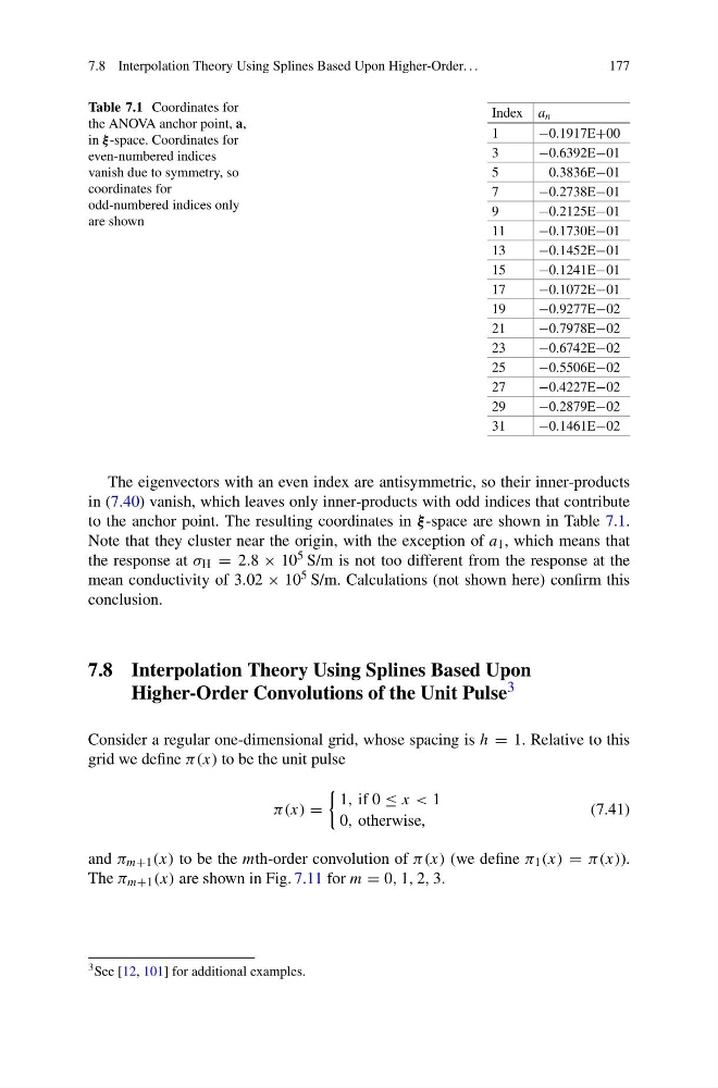
Table 7.1 Coordinates for
the ANOVA anchor point, a,
in ξ -space. Coordinates for
even-numbered indices
vanish due to symmetry, so
coordinates for
odd-numbered indices only
are shown
Index a n
1
−0.1917E+00
3
−0.6392E−01
5
0.3836E−01
7
−0.2738E−01
9
−0.2125E−01
11
−0.1730E−01
13
−0.1452E−01
15
−0.1241E−01
17
−0.1072E−01
19
−0.9277E−02
21
−0.7978E−02
23
−0.6742E−02
25
−0.5506E−02
27
−0.4227E−02
29
−0.2879E−02
31
−0.1461E−02
The eigenvectors with an even index are antisymmetric, so their inner-products
in (7.40) vanish, which leaves only inner-products with odd indices that contribute
to the anchor point. The resulting coordinates in ξ -space are shown in Table 7.1.
Note that they cluster near the origin, with the exception of a 1 , which means that
the response at σ H = 2.8 × 10 5 S/m is not too different from the response at the
mean conductivity of 3.02 × 10 5 S/m. Calculations (not shown here) confirm this
conclusion.
7.8 Interpolation Theory Using Splines Based Upon
Higher-Order Convolutions of the Unit Pulse 3
Consider a regular one-dimensional grid, whose spacing is h = 1. Relative to this
grid we define π(x) to be the unit pulse
π(x) =
1, if 0 ≤ x < 1
0, otherwise,
(7.41)
and π m+1 (x) to be the mth-order convolution of π(x) (we define π 1 (x) = π(x)).
The π m+1 (x) are shown in Fig. 7.11 for m = 0, 1, 2, 3.
3 See [12, 101] for additional examples.
177
Table 7.1 Coordinates for
the ANOVA anchor point, a,
in ξ -space. Coordinates for
even-numbered indices
vanish due to symmetry, so
coordinates for
odd-numbered indices only
are shown
Index a n
1
−0.1917E+00
3
−0.6392E−01
5
0.3836E−01
7
−0.2738E−01
9
−0.2125E−01
11
−0.1730E−01
13
−0.1452E−01
15
−0.1241E−01
17
−0.1072E−01
19
−0.9277E−02
21
−0.7978E−02
23
−0.6742E−02
25
−0.5506E−02
27
−0.4227E−02
29
−0.2879E−02
31
−0.1461E−02
The eigenvectors with an even index are antisymmetric, so their inner-products
in (7.40) vanish, which leaves only inner-products with odd indices that contribute
to the anchor point. The resulting coordinates in ξ -space are shown in Table 7.1.
Note that they cluster near the origin, with the exception of a 1 , which means that
the response at σ H = 2.8 × 10 5 S/m is not too different from the response at the
mean conductivity of 3.02 × 10 5 S/m. Calculations (not shown here) confirm this
conclusion.
7.8 Interpolation Theory Using Splines Based Upon
Higher-Order Convolutions of the Unit Pulse 3
Consider a regular one-dimensional grid, whose spacing is h = 1. Relative to this
grid we define π(x) to be the unit pulse
π(x) =
1, if 0 ≤ x < 1
0, otherwise,
(7.41)
and π m+1 (x) to be the mth-order convolution of π(x) (we define π 1 (x) = π(x)).
The π m+1 (x) are shown in Fig. 7.11 for m = 0, 1, 2, 3.
3 See [12, 101] for additional examples.