

7.5 gPC and PCM
169
-0.6
-0.4
-0.2
0
0.2
0.4
0.6
0.8
1
0
0.5
1
1.5
2
Ohms
Normalized Flaw Conductivity
Impedance as a function of normalized flaw conductivity
R
X
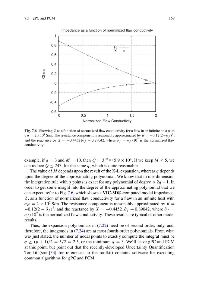
Fig. 7.6 Showing Z as a function of normalized flaw conductivity for a flaw in an infinite host with
σ H = 2×10 7 S/m. The resistance component is reasonably approximated by R = −0.12(2− ˆ
σ f ) 2 ,
and the reactance by X = −0.44521 ˆ
σ f + 0.89042, where ˆ
σ f = σ f /10 7 is the normalized flaw
conductivity
example, if q = 3 and M = 10, then Q = 3 10 ≈ 5.9 × 10 4 . If we keep M ≤ 5, we
can reduce Q ≤ 243, for the same q, which is quite reasonable.
The value of M depends upon the result of the K-L expansion, whereas q depends
upon the degree of the approximating polynomial. We know that in one dimension
the integration rule with q points is exact for any polynomial of degree ≤ 2q − 1. In
order to get some insight into the degree of the approximating polynomial that we
can expect, refer to Fig. 7.6, which shows a VIC-3D®-computed model impedance,
Z, as a function of normalized flaw conductivity for a flaw in an infinite host with
σ H = 2 × 10 7 S/m. The resistance component is reasonably approximated by R =
−0.12(2 − ˆ
σ f ) 2 , and the reactance by X = −0.44521 ˆ
σ f + 0.89042, where ˆ
σ f =
σ f /10 7 is the normalized flaw conductivity. These results are typical of other model
results.
Thus, the expansion polynomials in (7.22) need be of second order, only, and,
therefore, the integrands in (7.24) are at most fourth-order polynomials. From what
was just stated, the number of nodal points to exactly compute the integral must be
q ≥ (p + 1)/2 = 5/2 = 2.5, or the minimum q = 3. We’ll leave gPC and PCM
at this point, but point out that the recently-developed Uncertainty Quantification
Toolkit (see [33] for references to the toolkit) contains software for executing
common algorithms for gPC and PCM.
169
-0.6
-0.4
-0.2
0
0.2
0.4
0.6
0.8
1
0
0.5
1
1.5
2
Ohms
Normalized Flaw Conductivity
Impedance as a function of normalized flaw conductivity
R
X
Fig. 7.6 Showing Z as a function of normalized flaw conductivity for a flaw in an infinite host with
σ H = 2×10 7 S/m. The resistance component is reasonably approximated by R = −0.12(2− ˆ
σ f ) 2 ,
and the reactance by X = −0.44521 ˆ
σ f + 0.89042, where ˆ
σ f = σ f /10 7 is the normalized flaw
conductivity
example, if q = 3 and M = 10, then Q = 3 10 ≈ 5.9 × 10 4 . If we keep M ≤ 5, we
can reduce Q ≤ 243, for the same q, which is quite reasonable.
The value of M depends upon the result of the K-L expansion, whereas q depends
upon the degree of the approximating polynomial. We know that in one dimension
the integration rule with q points is exact for any polynomial of degree ≤ 2q − 1. In
order to get some insight into the degree of the approximating polynomial that we
can expect, refer to Fig. 7.6, which shows a VIC-3D®-computed model impedance,
Z, as a function of normalized flaw conductivity for a flaw in an infinite host with
σ H = 2 × 10 7 S/m. The resistance component is reasonably approximated by R =
−0.12(2 − ˆ
σ f ) 2 , and the reactance by X = −0.44521 ˆ
σ f + 0.89042, where ˆ
σ f =
σ f /10 7 is the normalized flaw conductivity. These results are typical of other model
results.
Thus, the expansion polynomials in (7.22) need be of second order, only, and,
therefore, the integrands in (7.24) are at most fourth-order polynomials. From what
was just stated, the number of nodal points to exactly compute the integral must be
q ≥ (p + 1)/2 = 5/2 = 2.5, or the minimum q = 3. We’ll leave gPC and PCM
at this point, but point out that the recently-developed Uncertainty Quantification
Toolkit (see [33] for references to the toolkit) contains software for executing
common algorithms for gPC and PCM.