

168
7 Integration of Functionals, PCM and Stochastic IntegralEquations
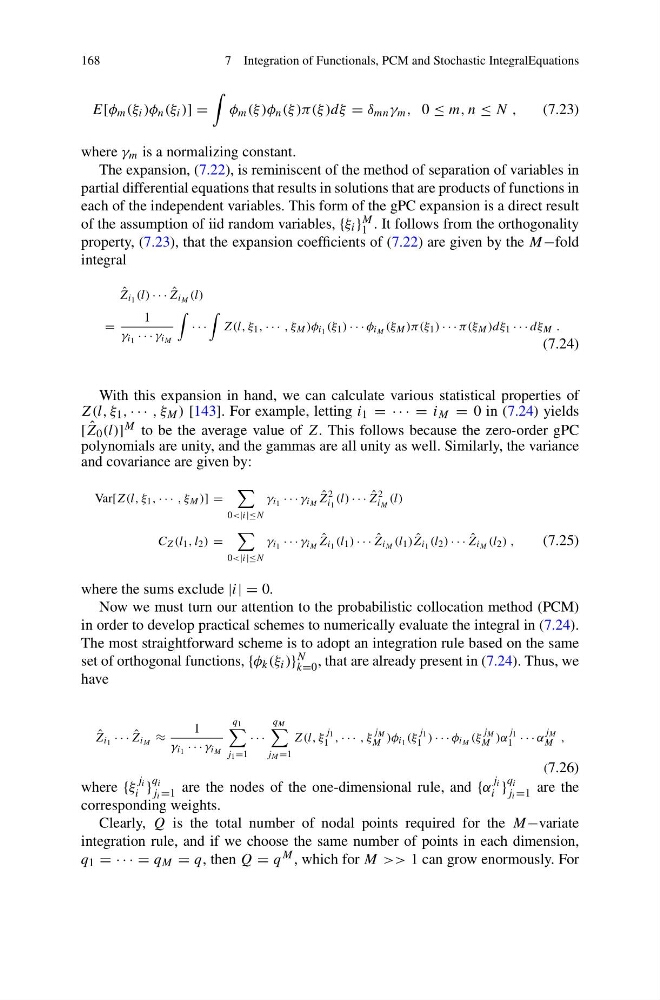
E[φ m (ξ i )φ n (ξ i )] =
φ m (ξ )φ n (ξ )π(ξ )dξ = δ mn γ m , 0 ≤ m, n ≤ N ,
(7.23)
where γ m is a normalizing constant.
The expansion, (7.22), is reminiscent of the method of separation of variables in
partial differential equations that results in solutions that are products of functions in
each of the independent variables. This form of the gPC expansion is a direct result
of the assumption of iid random variables, {ξ i } M
1 . It follows from the orthogonality
property, (7.23), that the expansion coefficients of (7.22) are given by the M−fold
integral
ˆ
Z i 1 (l) · · · ˆ
Z i M (l)
=
1
γ i 1 · · · γ i M
· · ·
Z(l, ξ 1 , · · · , ξ M )φ i 1 (ξ 1 ) · · · φ i M (ξ M )π(ξ 1 ) · · · π(ξ M )dξ 1 · · · dξ M .
(7.24)
With this expansion in hand, we can calculate various statistical properties of
Z(l, ξ 1 , · · · , ξ M ) [143]. For example, letting i 1 = · · · = i M = 0 in (7.24) yields
[ ˆ
Z 0 (l)] M to be the average value of Z. This follows because the zero-order gPC
polynomials are unity, and the gammas are all unity as well. Similarly, the variance
and covariance are given by:
Var[Z(l, ξ 1 , · · · , ξ M )] =
0<|i|≤N
γ i 1 · · · γ i M ˆ
Z
2
i 1
(l) · · · ˆ
Z
2
i M
(l)
C Z (l 1 , l 2 ) =
0<|i|≤N
γ i 1 · · · γ i M ˆ
Z i 1 (l 1 ) · · · ˆ
Z i M (l 1 ) ˆ
Z i 1 (l 2 ) · · · ˆ
Z i M (l 2 ) ,
(7.25)
where the sums exclude |i| = 0.
Now we must turn our attention to the probabilistic collocation method (PCM)
in order to develop practical schemes to numerically evaluate the integral in (7.24).
The most straightforward scheme is to adopt an integration rule based on the same
set of orthogonal functions, {φ k (ξ i )} N
k=0 , that are already present in (7.24). Thus, we
have
ˆ
Z i 1 · · · ˆ
Z i M ≈
1
γ i 1 · · · γ i M
q 1
j 1 =1
· · ·
q M
j M =1
Z(l, ξ
j 1
1 , · · · , ξ
j M
M )φ i 1 (ξ
j 1
1 ) · · · φ i M (ξ
j M
M )α
j 1
1 · · · α
j M
M ,
(7.26)
where {ξ
j i
i }
q i
j i =1 are the nodes of the one-dimensional rule, and {α
j i
i }
q i
j i =1 are the
corresponding weights.
Clearly, Q is the total number of nodal points required for the M−variate
integration rule, and if we choose the same number of points in each dimension,
q 1 = · · · = q M = q, then Q = q M , which for M >> 1 can grow enormously. For
7 Integration of Functionals, PCM and Stochastic IntegralEquations
E[φ m (ξ i )φ n (ξ i )] =
φ m (ξ )φ n (ξ )π(ξ )dξ = δ mn γ m , 0 ≤ m, n ≤ N ,
(7.23)
where γ m is a normalizing constant.
The expansion, (7.22), is reminiscent of the method of separation of variables in
partial differential equations that results in solutions that are products of functions in
each of the independent variables. This form of the gPC expansion is a direct result
of the assumption of iid random variables, {ξ i } M
1 . It follows from the orthogonality
property, (7.23), that the expansion coefficients of (7.22) are given by the M−fold
integral
ˆ
Z i 1 (l) · · · ˆ
Z i M (l)
=
1
γ i 1 · · · γ i M
· · ·
Z(l, ξ 1 , · · · , ξ M )φ i 1 (ξ 1 ) · · · φ i M (ξ M )π(ξ 1 ) · · · π(ξ M )dξ 1 · · · dξ M .
(7.24)
With this expansion in hand, we can calculate various statistical properties of
Z(l, ξ 1 , · · · , ξ M ) [143]. For example, letting i 1 = · · · = i M = 0 in (7.24) yields
[ ˆ
Z 0 (l)] M to be the average value of Z. This follows because the zero-order gPC
polynomials are unity, and the gammas are all unity as well. Similarly, the variance
and covariance are given by:
Var[Z(l, ξ 1 , · · · , ξ M )] =
0<|i|≤N
γ i 1 · · · γ i M ˆ
Z
2
i 1
(l) · · · ˆ
Z
2
i M
(l)
C Z (l 1 , l 2 ) =
0<|i|≤N
γ i 1 · · · γ i M ˆ
Z i 1 (l 1 ) · · · ˆ
Z i M (l 1 ) ˆ
Z i 1 (l 2 ) · · · ˆ
Z i M (l 2 ) ,
(7.25)
where the sums exclude |i| = 0.
Now we must turn our attention to the probabilistic collocation method (PCM)
in order to develop practical schemes to numerically evaluate the integral in (7.24).
The most straightforward scheme is to adopt an integration rule based on the same
set of orthogonal functions, {φ k (ξ i )} N
k=0 , that are already present in (7.24). Thus, we
have
ˆ
Z i 1 · · · ˆ
Z i M ≈
1
γ i 1 · · · γ i M
q 1
j 1 =1
· · ·
q M
j M =1
Z(l, ξ
j 1
1 , · · · , ξ
j M
M )φ i 1 (ξ
j 1
1 ) · · · φ i M (ξ
j M
M )α
j 1
1 · · · α
j M
M ,
(7.26)
where {ξ
j i
i }
q i
j i =1 are the nodes of the one-dimensional rule, and {α
j i
i }
q i
j i =1 are the
corresponding weights.
Clearly, Q is the total number of nodal points required for the M−variate
integration rule, and if we choose the same number of points in each dimension,
q 1 = · · · = q M = q, then Q = q M , which for M >> 1 can grow enormously. For