

5.1 Theory
131
Q
(zz)
mM =
⎧
⎪ ⎪ ⎪ ⎪ ⎪ ⎨
⎪ ⎪ ⎪ ⎪ ⎪ ⎩
σ
z
klm+1
2(σ
z
klm + σ
z
klm+1 )
if M = m − 1
1
i fM = m
σ
z
klm
2(σ
z
klm + σ
z
klm+1 )
if M = m + 1
(5.31)
Note that if the anomalous conductivity in two adjacent cells vanishes, then the
indeterminate terms in the Q ’s are equal to 1/4. Also, if the conductivity of
either cell (or both) vanishes, then the corresponding ν klm of (5.30) also vanishes.
This follows because the numerators of the ν’s vanish to a higher-order than the
denominators. The result is that the corresponding J KLM vanishes.
A Test Problem
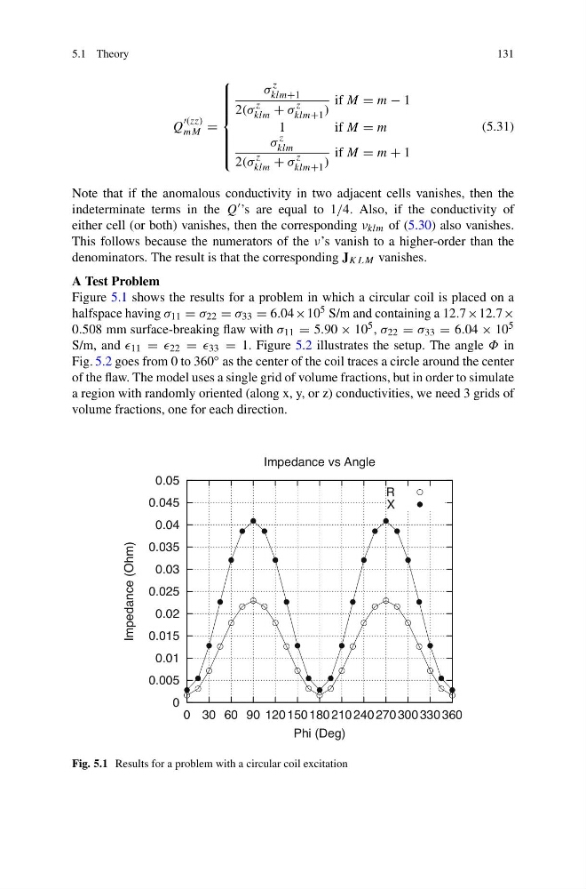
Figure 5.1 shows the results for a problem in which a circular coil is placed on a
halfspace having σ 11 = σ 22 = σ 33 = 6.04×10 5 S/m and containing a 12.7×12.7×
0.508 mm surface-breaking flaw with σ 11 = 5.90 × 10 5 , σ 22 = σ 33 = 6.04 × 10 5
S/m, and 11 = 22 = 33 = 1. Figure 5.2 illustrates the setup. The angle Φ in
Fig. 5.2 goes from 0 to 360 ◦ as the center of the coil traces a circle around the center
of the flaw. The model uses a single grid of volume fractions, but in order to simulate
a region with randomly oriented (along x, y, or z) conductivities, we need 3 grids of
volume fractions, one for each direction.
0
0.005
0.01
0.015
0.02
0.025
0.03
0.035
0.04
0.045
0.05
0 30 60 90 120 150 180 210 240 270 300 330 360
Impedance (Ohm)
Phi (Deg)
Impedance vs Angle
R
X
Fig. 5.1 Results for a problem with a circular coil excitation
131
Q
(zz)
mM =
⎧
⎪ ⎪ ⎪ ⎪ ⎪ ⎨
⎪ ⎪ ⎪ ⎪ ⎪ ⎩
σ
z
klm+1
2(σ
z
klm + σ
z
klm+1 )
if M = m − 1
1
i fM = m
σ
z
klm
2(σ
z
klm + σ
z
klm+1 )
if M = m + 1
(5.31)
Note that if the anomalous conductivity in two adjacent cells vanishes, then the
indeterminate terms in the Q ’s are equal to 1/4. Also, if the conductivity of
either cell (or both) vanishes, then the corresponding ν klm of (5.30) also vanishes.
This follows because the numerators of the ν’s vanish to a higher-order than the
denominators. The result is that the corresponding J KLM vanishes.
A Test Problem
Figure 5.1 shows the results for a problem in which a circular coil is placed on a
halfspace having σ 11 = σ 22 = σ 33 = 6.04×10 5 S/m and containing a 12.7×12.7×
0.508 mm surface-breaking flaw with σ 11 = 5.90 × 10 5 , σ 22 = σ 33 = 6.04 × 10 5
S/m, and 11 = 22 = 33 = 1. Figure 5.2 illustrates the setup. The angle Φ in
Fig. 5.2 goes from 0 to 360 ◦ as the center of the coil traces a circle around the center
of the flaw. The model uses a single grid of volume fractions, but in order to simulate
a region with randomly oriented (along x, y, or z) conductivities, we need 3 grids of
volume fractions, one for each direction.
0
0.005
0.01
0.015
0.02
0.025
0.03
0.035
0.04
0.045
0.05
0 30 60 90 120 150 180 210 240 270 300 330 360
Impedance (Ohm)
Phi (Deg)
Impedance vs Angle
R
X
Fig. 5.1 Results for a problem with a circular coil excitation