

5.1 Theory
129
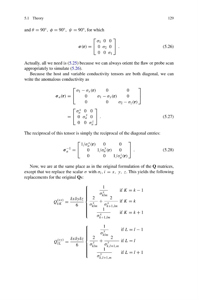
and θ = 90 ◦ , φ = 90 ◦ , ψ = 90 ◦ , for which
σ (r) =
⎡
⎣
σ 1 0 0
0 σ 2 0
0 0 σ 1
⎤
⎦ .
(5.26)
Actually, all we need is (5.25) because we can always orient the flaw or probe scan
appropriately to simulate (5.26).
Because the host and variable conductivity tensors are both diagonal, we can
write the anomalous conductivity as
σ a (r) =
⎡
⎣
σ 1 − σ x (r)
0
0
0
σ 1 − σ y (r)
0
0
0
σ 2 − σ z (r)
⎤
⎦
=
⎡
⎣
σ x
a 0 0
0 σ
y
a 0
0 0 σ z
a
⎤
⎦ .
(5.27)
The reciprocal of this tensor is simply the reciprocal of the diagonal entries:
σ
−1
a =
⎡
⎣
1/σ x
a (r)
0
0
0
1/σ
y
a (r)
0
0
0
1 /σ z
a (r)
⎤
⎦ .
(5.28)
Now, we are at the same place as in the original formulation of the Q matrices,
except that we replace the scalar σ with σ i , i = x, y, z. This yields the following
replacements for the original Qs:
Q
(xx)
kK =
δxδyδz
6
⎧
⎪ ⎪ ⎪ ⎪ ⎪ ⎪ ⎨
⎪ ⎪ ⎪ ⎪ ⎪ ⎪ ⎩
1
σ x
klm
if K = k − 1
2
σ x
klm
+
2
σ x
k+1,lm
if K = k
1
σ x
k+1,lm
if K = k + 1
Q
(yy)
lL =
δxδyδz
6
⎧
⎪ ⎪ ⎪ ⎪ ⎪ ⎪ ⎨
⎪ ⎪ ⎪ ⎪ ⎪ ⎪ ⎩
1
σ
y
klm
if L = l − 1
2
σ
y
klm
+
2
σ
y
k,l+1,m
if L = l
1
σ
y
k,l+1,m
if L = l + 1
129
and θ = 90 ◦ , φ = 90 ◦ , ψ = 90 ◦ , for which
σ (r) =
⎡
⎣
σ 1 0 0
0 σ 2 0
0 0 σ 1
⎤
⎦ .
(5.26)
Actually, all we need is (5.25) because we can always orient the flaw or probe scan
appropriately to simulate (5.26).
Because the host and variable conductivity tensors are both diagonal, we can
write the anomalous conductivity as
σ a (r) =
⎡
⎣
σ 1 − σ x (r)
0
0
0
σ 1 − σ y (r)
0
0
0
σ 2 − σ z (r)
⎤
⎦
=
⎡
⎣
σ x
a 0 0
0 σ
y
a 0
0 0 σ z
a
⎤
⎦ .
(5.27)
The reciprocal of this tensor is simply the reciprocal of the diagonal entries:
σ
−1
a =
⎡
⎣
1/σ x
a (r)
0
0
0
1/σ
y
a (r)
0
0
0
1 /σ z
a (r)
⎤
⎦ .
(5.28)
Now, we are at the same place as in the original formulation of the Q matrices,
except that we replace the scalar σ with σ i , i = x, y, z. This yields the following
replacements for the original Qs:
Q
(xx)
kK =
δxδyδz
6
⎧
⎪ ⎪ ⎪ ⎪ ⎪ ⎪ ⎨
⎪ ⎪ ⎪ ⎪ ⎪ ⎪ ⎩
1
σ x
klm
if K = k − 1
2
σ x
klm
+
2
σ x
k+1,lm
if K = k
1
σ x
k+1,lm
if K = k + 1
Q
(yy)
lL =
δxδyδz
6
⎧
⎪ ⎪ ⎪ ⎪ ⎪ ⎪ ⎨
⎪ ⎪ ⎪ ⎪ ⎪ ⎪ ⎩
1
σ
y
klm
if L = l − 1
2
σ
y
klm
+
2
σ
y
k,l+1,m
if L = l
1
σ
y
k,l+1,m
if L = l + 1