

5.1 Theory
127
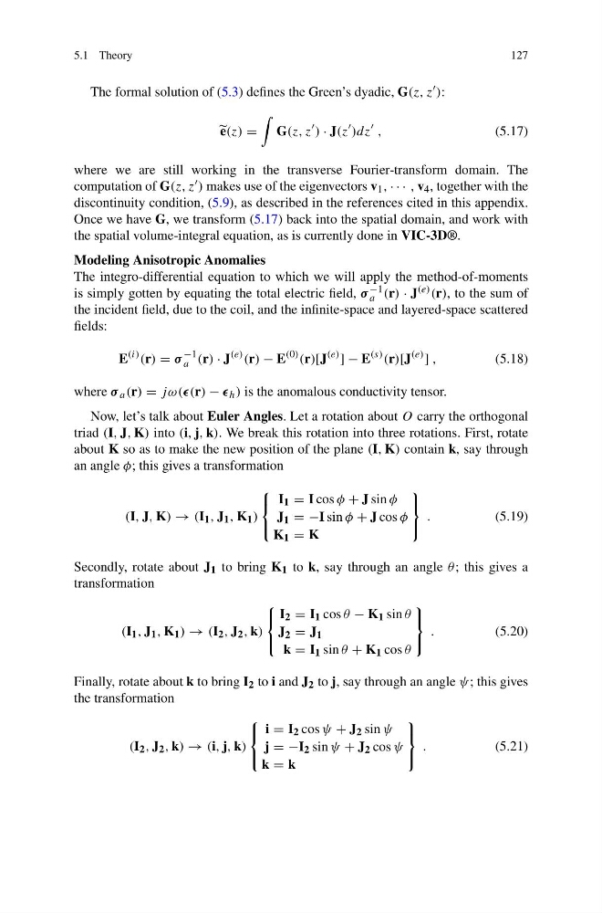
The formal solution of (5.3) defines the Green’s dyadic, G(z, z ):
e(z) =
G(z, z
) · J(z
)dz
,
(5.17)
where we are still working in the transverse Fourier-transform domain. The
computation of G(z, z ) makes use of the eigenvectors v 1 , · · · , v 4 , together with the
discontinuity condition, (5.9), as described in the references cited in this appendix.
Once we have G, we transform (5.17) back into the spatial domain, and work with
the spatial volume-integral equation, as is currently done in VIC-3D®.
Modeling Anisotropic Anomalies
The integro-differential equation to which we will apply the method-of-moments
is simply gotten by equating the total electric field, σ −1
a (r) · J (e) (r), to the sum of
the incident field, due to the coil, and the infinite-space and layered-space scattered
fields:
E
(i) (r) = σ
−1
a (r) · J
(e) (r) − E
(0) (r)[J
(e)
] − E
(s) (r)[J
(e)
] ,
(5.18)
where σ a (r) = jω((r) − h ) is the anomalous conductivity tensor.
Now, let’s talk about Euler Angles. Let a rotation about O carry the orthogonal
triad (I, J, K) into (i, j, k). We break this rotation into three rotations. First, rotate
about K so as to make the new position of the plane (I, K) contain k, say through
an angle φ; this gives a transformation
(I, J, K) → (I 1 , J 1 , K 1 )
⎧
⎨
⎩
I 1 = I cos φ + J sin φ
J 1 = −I sin φ + J cos φ
K 1 = K
⎫
⎬
⎭
.
(5.19)
Secondly, rotate about J 1 to bring K 1 to k, say through an angle θ ; this gives a
transformation
(I 1 , J 1 , K 1 ) → (I 2 , J 2 , k)
⎧
⎨
⎩
I 2 = I 1 cos θ − K 1 sin θ
J 2 = J 1
k = I 1 sin θ + K 1 cos θ
⎫
⎬
⎭
.
(5.20)
Finally, rotate about k to bring I 2 to i and J 2 to j, say through an angle ψ; this gives
the transformation
(I 2 , J 2 , k) → (i, j, k)
⎧
⎨
⎩
i = I 2 cos ψ + J 2 sin ψ
j = −I 2 sin ψ + J 2 cos ψ
k = k
⎫
⎬
⎭
.
(5.21)
127
The formal solution of (5.3) defines the Green’s dyadic, G(z, z ):
e(z) =
G(z, z
) · J(z
)dz
,
(5.17)
where we are still working in the transverse Fourier-transform domain. The
computation of G(z, z ) makes use of the eigenvectors v 1 , · · · , v 4 , together with the
discontinuity condition, (5.9), as described in the references cited in this appendix.
Once we have G, we transform (5.17) back into the spatial domain, and work with
the spatial volume-integral equation, as is currently done in VIC-3D®.
Modeling Anisotropic Anomalies
The integro-differential equation to which we will apply the method-of-moments
is simply gotten by equating the total electric field, σ −1
a (r) · J (e) (r), to the sum of
the incident field, due to the coil, and the infinite-space and layered-space scattered
fields:
E
(i) (r) = σ
−1
a (r) · J
(e) (r) − E
(0) (r)[J
(e)
] − E
(s) (r)[J
(e)
] ,
(5.18)
where σ a (r) = jω((r) − h ) is the anomalous conductivity tensor.
Now, let’s talk about Euler Angles. Let a rotation about O carry the orthogonal
triad (I, J, K) into (i, j, k). We break this rotation into three rotations. First, rotate
about K so as to make the new position of the plane (I, K) contain k, say through
an angle φ; this gives a transformation
(I, J, K) → (I 1 , J 1 , K 1 )
⎧
⎨
⎩
I 1 = I cos φ + J sin φ
J 1 = −I sin φ + J cos φ
K 1 = K
⎫
⎬
⎭
.
(5.19)
Secondly, rotate about J 1 to bring K 1 to k, say through an angle θ ; this gives a
transformation
(I 1 , J 1 , K 1 ) → (I 2 , J 2 , k)
⎧
⎨
⎩
I 2 = I 1 cos θ − K 1 sin θ
J 2 = J 1
k = I 1 sin θ + K 1 cos θ
⎫
⎬
⎭
.
(5.20)
Finally, rotate about k to bring I 2 to i and J 2 to j, say through an angle ψ; this gives
the transformation
(I 2 , J 2 , k) → (i, j, k)
⎧
⎨
⎩
i = I 2 cos ψ + J 2 sin ψ
j = −I 2 sin ψ + J 2 cos ψ
k = k
⎫
⎬
⎭
.
(5.21)