

76
4 Scalable Interdigitated Photoconductive Emitters for the Electrical …
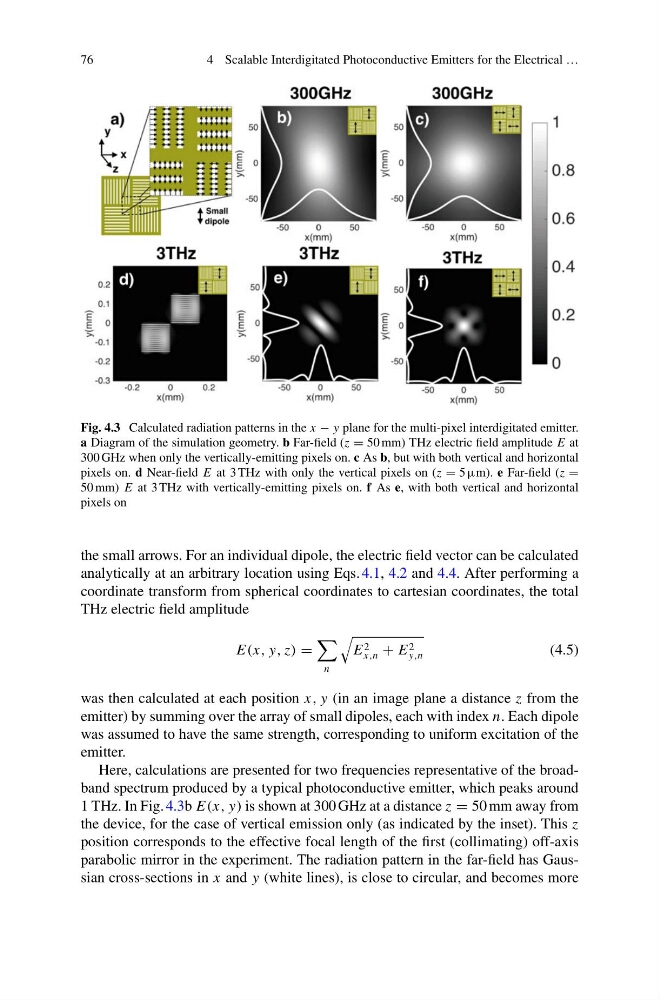
Fig. 4.3 Calculated radiation patterns in the x − y plane for the multi-pixel interdigitated emitter.
a Diagram of the simulation geometry. b Far-field (z = 50 mm) THz electric field amplitude E at
300 GHz when only the vertically-emitting pixels on. c As b, but with both vertical and horizontal
pixels on. d Near-field E at 3 THz with only the vertical pixels on (z = 5 µm). e Far-field (z =
50 mm) E at 3 THz with vertically-emitting pixels on. f As e, with both vertical and horizontal
pixels on
the small arrows. For an individual dipole, the electric field vector can be calculated
analytically at an arbitrary location using Eqs. 4.1, 4.2 and 4.4. After performing a
coordinate transform from spherical coordinates to cartesian coordinates, the total
THz electric field amplitude
E(x, y, z) =
n
E 2
x,n + E 2
y,n
(4.5)
was then calculated at each position x, y (in an image plane a distance z from the
emitter) by summing over the array of small dipoles, each with index n. Each dipole
was assumed to have the same strength, corresponding to uniform excitation of the
emitter.
Here, calculations are presented for two frequencies representative of the broadband spectrum produced by a typical photoconductive emitter, which peaks around
1 THz. In Fig. 4.3b E(x, y) is shown at 300 GHz at a distance z = 50 mm away from
the device, for the case of vertical emission only (as indicated by the inset). This z
position corresponds to the effective focal length of the first (collimating) off-axis
parabolic mirror in the experiment. The radiation pattern in the far-field has Gaussian cross-sections in x and y (white lines), is close to circular, and becomes more
4 Scalable Interdigitated Photoconductive Emitters for the Electrical …
Fig. 4.3 Calculated radiation patterns in the x − y plane for the multi-pixel interdigitated emitter.
a Diagram of the simulation geometry. b Far-field (z = 50 mm) THz electric field amplitude E at
300 GHz when only the vertically-emitting pixels on. c As b, but with both vertical and horizontal
pixels on. d Near-field E at 3 THz with only the vertical pixels on (z = 5 µm). e Far-field (z =
50 mm) E at 3 THz with vertically-emitting pixels on. f As e, with both vertical and horizontal
pixels on
the small arrows. For an individual dipole, the electric field vector can be calculated
analytically at an arbitrary location using Eqs. 4.1, 4.2 and 4.4. After performing a
coordinate transform from spherical coordinates to cartesian coordinates, the total
THz electric field amplitude
E(x, y, z) =
n
E 2
x,n + E 2
y,n
(4.5)
was then calculated at each position x, y (in an image plane a distance z from the
emitter) by summing over the array of small dipoles, each with index n. Each dipole
was assumed to have the same strength, corresponding to uniform excitation of the
emitter.
Here, calculations are presented for two frequencies representative of the broadband spectrum produced by a typical photoconductive emitter, which peaks around
1 THz. In Fig. 4.3b E(x, y) is shown at 300 GHz at a distance z = 50 mm away from
the device, for the case of vertical emission only (as indicated by the inset). This z
position corresponds to the effective focal length of the first (collimating) off-axis
parabolic mirror in the experiment. The radiation pattern in the far-field has Gaussian cross-sections in x and y (white lines), is close to circular, and becomes more