

Darjeeling experiences highest CH 4 values during October–November, while Pondicherry at the southeastern
coastal site and Port Blair in Andaman Islands register
comparatively lower values (Lin et al. 2015). A dense
observational network is required for understanding the
spatial and temporal variations of CH 4 over India, in particular the central Indian region which is characterized by
sparse and intermittent observational network. Chandra et al.
(2017) studied the variability of column dry-air mole fractions of methane (XCH 4 ) over India using GOSAT satellite
retrievals. The satellite observation of the XCH 4 is an integrated measure of CH 4 densities at all altitudes from the
surface to the top of the atmosphere. The Indian region was
divided into eight subregions, and relationship between
XCH 4 variability from surface to the upper troposphere with
the surface emissions was discussed. More often, the XCH 4
variabilities are strongly linked with the transport of air mass
from outside the domain of interests and monsoon anticyclone in the middle–upper troposphere. Variations of XCH 4
are controlled by both surface emissions and atmospheric
transport largely driven by the monsoonal dynamics. Various observational techniques have been used to make estimates of top-down CH 4 emissions in India (Schuck et al.
2010; Ganesan et al. 2013; Parker et al. 2015). It was shown
that there is a little growth in the CH 4 emissions in India
during the period 2010–2015. The reported emissions in
Ganesan et al. (2017) are 30% lower than the bottom-up
global inventory Emission Database for Global Atmospheric
-1
H
C
n
a
i
d
n
I
r
y
g
T
(
n
o
i
s
s
i
m
e
)
4
Prior (EDGAR excl. rice + Yan et al. + rice, GFED)
EDGAR incl. rice + GFED
Top-down (this study)
12-month running mean
First Biennial Update Report to the UNFCC
[b]
o
Longitude ( E)
o
)
N
(
e
d
u
t
i
t
a
L
[a]
2010
50
40
30
20
10
0
2011
2012
2013
2014
2015
60
10
20
30
40
70
80
90
100
110
GOSAT
CARIBIC
SNG
CRI
DJI
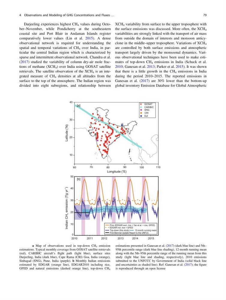
Fig. 4.4 a Map of observations used in top-down CH 4 emission
estimations. Typical monthly coverage from GOSAT satellite retrievals
(red), CARIBIC aircraft’s flight path (light blue), surface sites
Darjeeling, India (dark blue), Cape Rama (CRI) Goa, India (orange),
Sinhagad (SNG), Pune, India (purple). b Monthly Indian emissions
estimated by EDGAR (orange line), EDGAR2010 including rice,
GFED and natural emissions (dashed orange line), top-down CH 4
estimations presented in Ganesan et al. (2017) (dark blue line) and 5th–
95th percentile range (dark blue line shading), 12-month running mean
along with the 5th–95th percentile range of the running mean from this
study (light blue line and shading, respectively), 2010 emissions
submitted to the UNFCCC by Government of India (solid black line
and uncertainties as shaded line). Ref: Ganesan et al. (2017); the figure
is reproduced through an open license
4 Observations and Modeling of GHG Concentrations and Fluxes …
79
coastal site and Port Blair in Andaman Islands register
comparatively lower values (Lin et al. 2015). A dense
observational network is required for understanding the
spatial and temporal variations of CH 4 over India, in particular the central Indian region which is characterized by
sparse and intermittent observational network. Chandra et al.
(2017) studied the variability of column dry-air mole fractions of methane (XCH 4 ) over India using GOSAT satellite
retrievals. The satellite observation of the XCH 4 is an integrated measure of CH 4 densities at all altitudes from the
surface to the top of the atmosphere. The Indian region was
divided into eight subregions, and relationship between
XCH 4 variability from surface to the upper troposphere with
the surface emissions was discussed. More often, the XCH 4
variabilities are strongly linked with the transport of air mass
from outside the domain of interests and monsoon anticyclone in the middle–upper troposphere. Variations of XCH 4
are controlled by both surface emissions and atmospheric
transport largely driven by the monsoonal dynamics. Various observational techniques have been used to make estimates of top-down CH 4 emissions in India (Schuck et al.
2010; Ganesan et al. 2013; Parker et al. 2015). It was shown
that there is a little growth in the CH 4 emissions in India
during the period 2010–2015. The reported emissions in
Ganesan et al. (2017) are 30% lower than the bottom-up
global inventory Emission Database for Global Atmospheric
-1
H
C
n
a
i
d
n
I
r
y
g
T
(
n
o
i
s
s
i
m
e
)
4
Prior (EDGAR excl. rice + Yan et al. + rice, GFED)
EDGAR incl. rice + GFED
Top-down (this study)
12-month running mean
First Biennial Update Report to the UNFCC
[b]
o
Longitude ( E)
o
)
N
(
e
d
u
t
i
t
a
L
[a]
2010
50
40
30
20
10
0
2011
2012
2013
2014
2015
60
10
20
30
40
70
80
90
100
110
GOSAT
CARIBIC
SNG
CRI
DJI
Fig. 4.4 a Map of observations used in top-down CH 4 emission
estimations. Typical monthly coverage from GOSAT satellite retrievals
(red), CARIBIC aircraft’s flight path (light blue), surface sites
Darjeeling, India (dark blue), Cape Rama (CRI) Goa, India (orange),
Sinhagad (SNG), Pune, India (purple). b Monthly Indian emissions
estimated by EDGAR (orange line), EDGAR2010 including rice,
GFED and natural emissions (dashed orange line), top-down CH 4
estimations presented in Ganesan et al. (2017) (dark blue line) and 5th–
95th percentile range (dark blue line shading), 12-month running mean
along with the 5th–95th percentile range of the running mean from this
study (light blue line and shading, respectively), 2010 emissions
submitted to the UNFCCC by Government of India (solid black line
and uncertainties as shaded line). Ref: Ganesan et al. (2017); the figure
is reproduced through an open license
4 Observations and Modeling of GHG Concentrations and Fluxes …
79