

84
7 Regression Models and Hypothesis Testing
In this section, we determined the range that contains the “true” mean μ of a
distribution with a certain level of confidence. In the next section we will address a
related problem: the validation or rejection of a hypothesis about the value a parameter
is expected to have.
7.6 Hypothesis Testing and p-Values
In a regression analysis we might wonder whether we really need to include a certain
fit parameter ˆ
X or whether the model works equally well when omitting it. We can
address this problem by testing the hypothesis ˆ
X = 0. In particular, we reject the
hypothesis ˆ
X = 0 if the test-statistics t = X/σ (X ) is very large and lies in the tails
of the distribution. Here X is the value of a fitted parameter from (7.5) and σ (X ) is
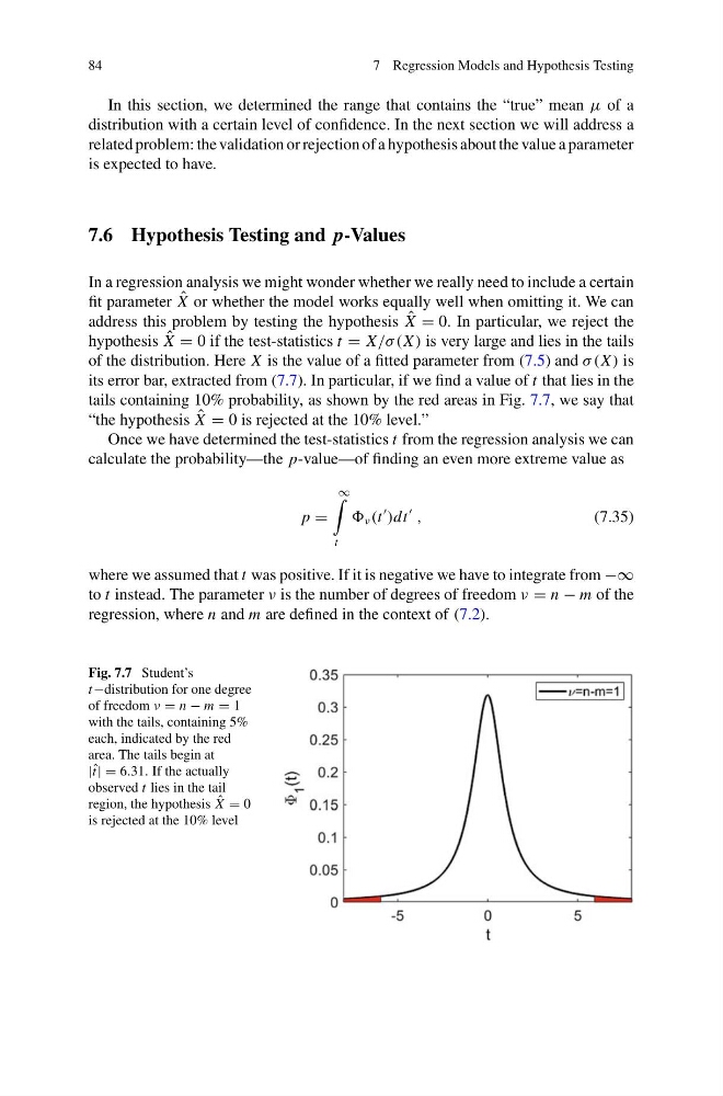
its error bar, extracted from (7.7). In particular, if we find a value of t that lies in the
tails containing 10% probability, as shown by the red areas in Fig. 7.7, we say that
“the hypothesis ˆ
X = 0 is rejected at the 10% level.”
Once we have determined the test-statistics t from the regression analysis we can
calculate the probability—the p-value—of finding an even more extreme value as
p =
∞
t
ν (t
)dt
,
(7.35)
where we assumed that t was positive. If it is negative we have to integrate from −∞
to t instead. The parameter ν is the number of degrees of freedom ν = n − m of the
regression, where n and m are defined in the context of (7.2).
Fig. 7.7 Student’s
t−distribution for one degree
of freedom ν = n − m = 1
with the tails, containing 5%
each, indicated by the red
area. The tails begin at
|ˆ t| = 6.31. If the actually
observed t lies in the tail
region, the hypothesis ˆ
X = 0
is rejected at the 10% level
7 Regression Models and Hypothesis Testing
In this section, we determined the range that contains the “true” mean μ of a
distribution with a certain level of confidence. In the next section we will address a
related problem: the validation or rejection of a hypothesis about the value a parameter
is expected to have.
7.6 Hypothesis Testing and p-Values
In a regression analysis we might wonder whether we really need to include a certain
fit parameter ˆ
X or whether the model works equally well when omitting it. We can
address this problem by testing the hypothesis ˆ
X = 0. In particular, we reject the
hypothesis ˆ
X = 0 if the test-statistics t = X/σ (X ) is very large and lies in the tails
of the distribution. Here X is the value of a fitted parameter from (7.5) and σ (X ) is
its error bar, extracted from (7.7). In particular, if we find a value of t that lies in the
tails containing 10% probability, as shown by the red areas in Fig. 7.7, we say that
“the hypothesis ˆ
X = 0 is rejected at the 10% level.”
Once we have determined the test-statistics t from the regression analysis we can
calculate the probability—the p-value—of finding an even more extreme value as
p =
∞
t
ν (t
)dt
,
(7.35)
where we assumed that t was positive. If it is negative we have to integrate from −∞
to t instead. The parameter ν is the number of degrees of freedom ν = n − m of the
regression, where n and m are defined in the context of (7.2).
Fig. 7.7 Student’s
t−distribution for one degree
of freedom ν = n − m = 1
with the tails, containing 5%
each, indicated by the red
area. The tails begin at
|ˆ t| = 6.31. If the actually
observed t lies in the tail
region, the hypothesis ˆ
X = 0
is rejected at the 10% level