

7.1 Regression and Linear Fitting
71
following form
⎛
⎜
⎜
⎜
⎝
y 1
y 2
. . .
y n
⎞
⎟
⎟
⎟
⎠
=
⎛
⎜
⎜
⎜
⎝
A 11 A 12 . . . A 1m
A 21 A 22 . . . A 2m
. . .
. . .
. . .
. . .
A n1 A n2 . . . A nm
⎞
⎟
⎟
⎟
⎠
⎛
⎜
⎜
⎜
⎝
x 1
x 2
. . .
x m
⎞
⎟
⎟
⎟
⎠
+
⎛
⎜
⎜
⎜
⎝
y 1
y 2
. . .
y n
⎞
⎟
⎟
⎟
⎠
,
(7.2)
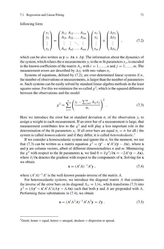
which can be also written as y = Ax + y. The information about the dynamics of
the system, which relates the n measurements y i to the m fit parameters x j , is encoded
in the known coefficients of the matrix A i j with i = 1, . . . , n and j = 1, . . . , m. The
measurement errors are described by y i with rms values σ i .
Systems of equations, defined by (7.2), are over-determined linear systems if n,
the number of observations or measurements, is larger than the number of parameters
m. Such systems can be easily solved by standard linear-algebra methods in the least
squares sense. For this we minimize the so-called χ
2 , which is the squared difference
between the observations and the model
χ
2
=
n
i=1
y i −
m
j=1 A i j x j
σ i
2
.
(7.3)
Here we introduce the error bar or standard deviation σ i of the observation y i to
assign a weight to each measurement. If an error bar of a measurement is large, that
measurement contributes less to the χ
2 and will play a less important role in the
determination of the fit parameters x i . If all error bars are equal σ i = σ for all i the
system is called homoscedastic and if they differ, it is called heteroskedastic.
1
If we consider a homoscedastic system and ignore the σ i for the moment, we see
that (7.3) can be written as a matrix equation χ
2
= (y
t
− x
t A
t
)(y − Ax), where x
and y are column vectors, albeit of different dimensionalities n and m. Minimizing
the χ
2 with respect to the fit parameters x, we find 0 = ∂χ
2
/∂x = −2 A
t
(y − Ax),
where ∂/∂x denotes the gradient with respect to the components of x. Solving for x
we obtain
x = (A
t A)
−1 A
t y ,
(7.4)
where (A
t A)
−1 A
t is the well-known pseudo-inverse of the matrix A.
For heteroscedastic systems, we introduce the diagonal matrix that contains
the inverse of the error bars on its diagonal ii = 1/σ i , which transforms (7.3) into
χ
2
= ((y
t
− x
t A
t
t
)((y − Ax) such that both y and A are prepended with .
Performing these substitutions in (7.4), we obtain
x = (A
t
2 A)
−1 A
t
2 y = J y .
(7.5)
1 Greek: homo = equal, hetero = unequal, skedasis = dispersion or spread.
71
following form
⎛
⎜
⎜
⎜
⎝
y 1
y 2
. . .
y n
⎞
⎟
⎟
⎟
⎠
=
⎛
⎜
⎜
⎜
⎝
A 11 A 12 . . . A 1m
A 21 A 22 . . . A 2m
. . .
. . .
. . .
. . .
A n1 A n2 . . . A nm
⎞
⎟
⎟
⎟
⎠
⎛
⎜
⎜
⎜
⎝
x 1
x 2
. . .
x m
⎞
⎟
⎟
⎟
⎠
+
⎛
⎜
⎜
⎜
⎝
y 1
y 2
. . .
y n
⎞
⎟
⎟
⎟
⎠
,
(7.2)
which can be also written as y = Ax + y. The information about the dynamics of
the system, which relates the n measurements y i to the m fit parameters x j , is encoded
in the known coefficients of the matrix A i j with i = 1, . . . , n and j = 1, . . . , m. The
measurement errors are described by y i with rms values σ i .
Systems of equations, defined by (7.2), are over-determined linear systems if n,
the number of observations or measurements, is larger than the number of parameters
m. Such systems can be easily solved by standard linear-algebra methods in the least
squares sense. For this we minimize the so-called χ
2 , which is the squared difference
between the observations and the model
χ
2
=
n
i=1
y i −
m
j=1 A i j x j
σ i
2
.
(7.3)
Here we introduce the error bar or standard deviation σ i of the observation y i to
assign a weight to each measurement. If an error bar of a measurement is large, that
measurement contributes less to the χ
2 and will play a less important role in the
determination of the fit parameters x i . If all error bars are equal σ i = σ for all i the
system is called homoscedastic and if they differ, it is called heteroskedastic.
1
If we consider a homoscedastic system and ignore the σ i for the moment, we see
that (7.3) can be written as a matrix equation χ
2
= (y
t
− x
t A
t
)(y − Ax), where x
and y are column vectors, albeit of different dimensionalities n and m. Minimizing
the χ
2 with respect to the fit parameters x, we find 0 = ∂χ
2
/∂x = −2 A
t
(y − Ax),
where ∂/∂x denotes the gradient with respect to the components of x. Solving for x
we obtain
x = (A
t A)
−1 A
t y ,
(7.4)
where (A
t A)
−1 A
t is the well-known pseudo-inverse of the matrix A.
For heteroscedastic systems, we introduce the diagonal matrix that contains
the inverse of the error bars on its diagonal ii = 1/σ i , which transforms (7.3) into
χ
2
= ((y
t
− x
t A
t
t
)((y − Ax) such that both y and A are prepended with .
Performing these substitutions in (7.4), we obtain
x = (A
t
2 A)
−1 A
t
2 y = J y .
(7.5)
1 Greek: homo = equal, hetero = unequal, skedasis = dispersion or spread.