

70
7 Regression Models and Hypothesis Testing
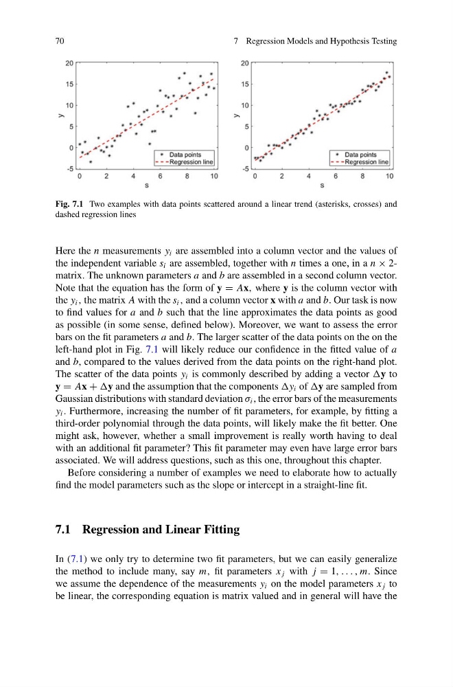
Fig. 7.1 Two examples with data points scattered around a linear trend (asterisks, crosses) and
dashed regression lines
Here the n measurements y i are assembled into a column vector and the values of
the independent variable s i are assembled, together with n times a one, in a n × 2matrix. The unknown parameters a and b are assembled in a second column vector.
Note that the equation has the form of y = Ax, where y is the column vector with
the y i , the matrix A with the s i , and a column vector x with a and b. Our task is now
to find values for a and b such that the line approximates the data points as good
as possible (in some sense, defined below). Moreover, we want to assess the error
bars on the fit parameters a and b. The larger scatter of the data points on the on the
left-hand plot in Fig. 7.1 will likely reduce our confidence in the fitted value of a
and b, compared to the values derived from the data points on the right-hand plot.
The scatter of the data points y i is commonly described by adding a vector y to
y = Ax + y and the assumption that the components y i of y are sampled from
Gaussian distributions with standard deviation σ i , the error bars of the measurements
y i . Furthermore, increasing the number of fit parameters, for example, by fitting a
third-order polynomial through the data points, will likely make the fit better. One
might ask, however, whether a small improvement is really worth having to deal
with an additional fit parameter? This fit parameter may even have large error bars
associated. We will address questions, such as this one, throughout this chapter.
Before considering a number of examples we need to elaborate how to actually
find the model parameters such as the slope or intercept in a straight-line fit.
7.1 Regression and Linear Fitting
In (7.1) we only try to determine two fit parameters, but we can easily generalize
the method to include many, say m, fit parameters x j with j = 1, . . . , m. Since
we assume the dependence of the measurements y i on the model parameters x j to
be linear, the corresponding equation is matrix valued and in general will have the
7 Regression Models and Hypothesis Testing
Fig. 7.1 Two examples with data points scattered around a linear trend (asterisks, crosses) and
dashed regression lines
Here the n measurements y i are assembled into a column vector and the values of
the independent variable s i are assembled, together with n times a one, in a n × 2matrix. The unknown parameters a and b are assembled in a second column vector.
Note that the equation has the form of y = Ax, where y is the column vector with
the y i , the matrix A with the s i , and a column vector x with a and b. Our task is now
to find values for a and b such that the line approximates the data points as good
as possible (in some sense, defined below). Moreover, we want to assess the error
bars on the fit parameters a and b. The larger scatter of the data points on the on the
left-hand plot in Fig. 7.1 will likely reduce our confidence in the fitted value of a
and b, compared to the values derived from the data points on the right-hand plot.
The scatter of the data points y i is commonly described by adding a vector y to
y = Ax + y and the assumption that the components y i of y are sampled from
Gaussian distributions with standard deviation σ i , the error bars of the measurements
y i . Furthermore, increasing the number of fit parameters, for example, by fitting a
third-order polynomial through the data points, will likely make the fit better. One
might ask, however, whether a small improvement is really worth having to deal
with an additional fit parameter? This fit parameter may even have large error bars
associated. We will address questions, such as this one, throughout this chapter.
Before considering a number of examples we need to elaborate how to actually
find the model parameters such as the slope or intercept in a straight-line fit.
7.1 Regression and Linear Fitting
In (7.1) we only try to determine two fit parameters, but we can easily generalize
the method to include many, say m, fit parameters x j with j = 1, . . . , m. Since
we assume the dependence of the measurements y i on the model parameters x j to
be linear, the corresponding equation is matrix valued and in general will have the