

24
3 Portfolio Theory and CAPM
Note that all points on the capital market line constitute the most efficient portfolios, and are convex combinations of investing a fraction of ones wealth in the
risk-free asset and the rest in the tangent portfolio, which incidentally is the same
as the market portfolio discussed in the beginning of this section. That all efficient
portfolios on the capital market line are linear combinations of just two investment
assets was first found by Tobin [4] and was called separation theorem.
In order to compare a previously unknown asset with the market, we can calculate
its Sharpe ratio and compare it to that of the market. If it is higher, the new asset
is worth buying. This is equivalent of placing the new asset in the diagram with the
portfolio space Fig. 3.2, where the properly valued assets should lie close to the (red)
capital market line. If stocks lie above the line, they are undervalued and constitute
a potential investment option. Conversely, if they lie below the capital market line,
they are over-valued and provide too little return for the risk that investing in them
would entail.
In the following section we discuss a slightly more refined method to figure out
whether we want to include a new asset in a portfolio.
3.5 Capital Asset Pricing Model
The Capital asset pricing model or CAPM, as it is known, describes the expected
return r 1 of an asset, that was not previously included in a portfolio, here the market
portfolio. The model was initially introduced by Sharpe [5] and Lintner [6]. Since
any efficient portfolio can be expressed as a sum of the risk-free asset and the market
portfolio, we consider a market with these three assets. All information about this
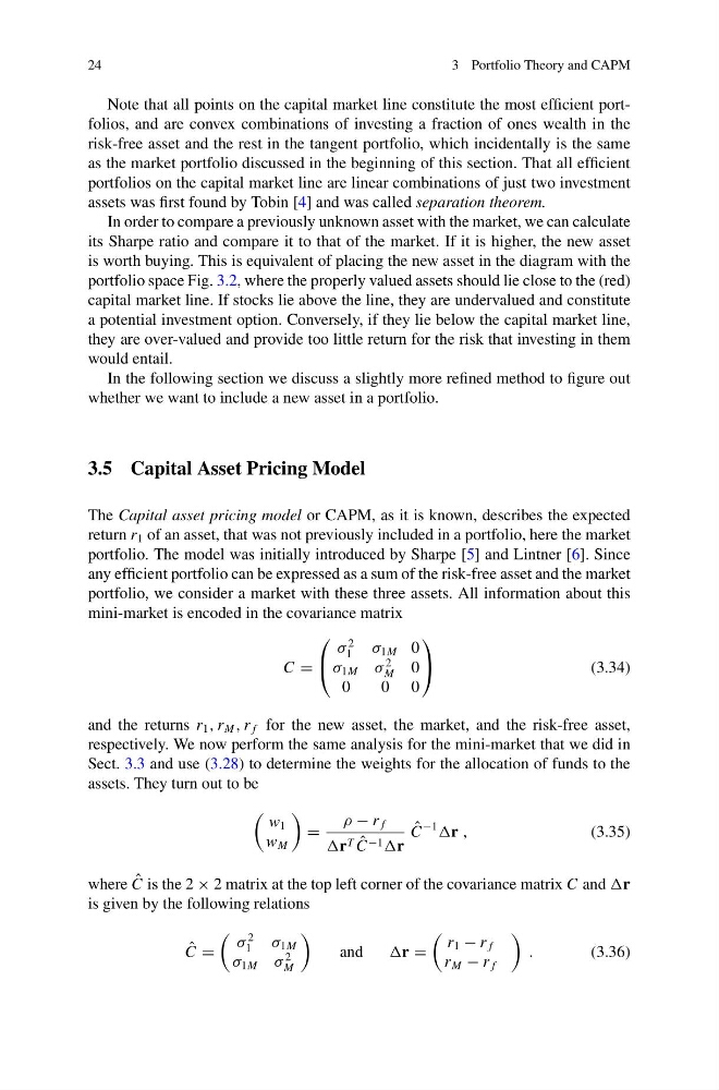
mini-market is encoded in the covariance matrix
C =
⎛
⎝
σ
2
1
σ 1M 0
σ 1M σ
2
M
0
0
0 0
⎞
⎠
(3.34)
and the returns r 1 , r M , r f for the new asset, the market, and the risk-free asset,
respectively. We now perform the same analysis for the mini-market that we did in
Sect. 3.3 and use (3.28) to determine the weights for the allocation of funds to the
assets. They turn out to be
w 1
w M
=
ρ − r f
r T ˆ
C −1 r
ˆ
C
−1
r ,
(3.35)
where ˆ
C is the 2 × 2 matrix at the top left corner of the covariance matrix C and r
is given by the following relations
ˆ
C =
σ
2
1
σ 1M
σ 1M σ
2
M
and
r =
r 1 − r f
r M − r f
.
(3.36)
3 Portfolio Theory and CAPM
Note that all points on the capital market line constitute the most efficient portfolios, and are convex combinations of investing a fraction of ones wealth in the
risk-free asset and the rest in the tangent portfolio, which incidentally is the same
as the market portfolio discussed in the beginning of this section. That all efficient
portfolios on the capital market line are linear combinations of just two investment
assets was first found by Tobin [4] and was called separation theorem.
In order to compare a previously unknown asset with the market, we can calculate
its Sharpe ratio and compare it to that of the market. If it is higher, the new asset
is worth buying. This is equivalent of placing the new asset in the diagram with the
portfolio space Fig. 3.2, where the properly valued assets should lie close to the (red)
capital market line. If stocks lie above the line, they are undervalued and constitute
a potential investment option. Conversely, if they lie below the capital market line,
they are over-valued and provide too little return for the risk that investing in them
would entail.
In the following section we discuss a slightly more refined method to figure out
whether we want to include a new asset in a portfolio.
3.5 Capital Asset Pricing Model
The Capital asset pricing model or CAPM, as it is known, describes the expected
return r 1 of an asset, that was not previously included in a portfolio, here the market
portfolio. The model was initially introduced by Sharpe [5] and Lintner [6]. Since
any efficient portfolio can be expressed as a sum of the risk-free asset and the market
portfolio, we consider a market with these three assets. All information about this
mini-market is encoded in the covariance matrix
C =
⎛
⎝
σ
2
1
σ 1M 0
σ 1M σ
2
M
0
0
0 0
⎞
⎠
(3.34)
and the returns r 1 , r M , r f for the new asset, the market, and the risk-free asset,
respectively. We now perform the same analysis for the mini-market that we did in
Sect. 3.3 and use (3.28) to determine the weights for the allocation of funds to the
assets. They turn out to be
w 1
w M
=
ρ − r f
r T ˆ
C −1 r
ˆ
C
−1
r ,
(3.35)
where ˆ
C is the 2 × 2 matrix at the top left corner of the covariance matrix C and r
is given by the following relations
ˆ
C =
σ
2
1
σ 1M
σ 1M σ
2
M
and
r =
r 1 − r f
r M − r f
.
(3.36)