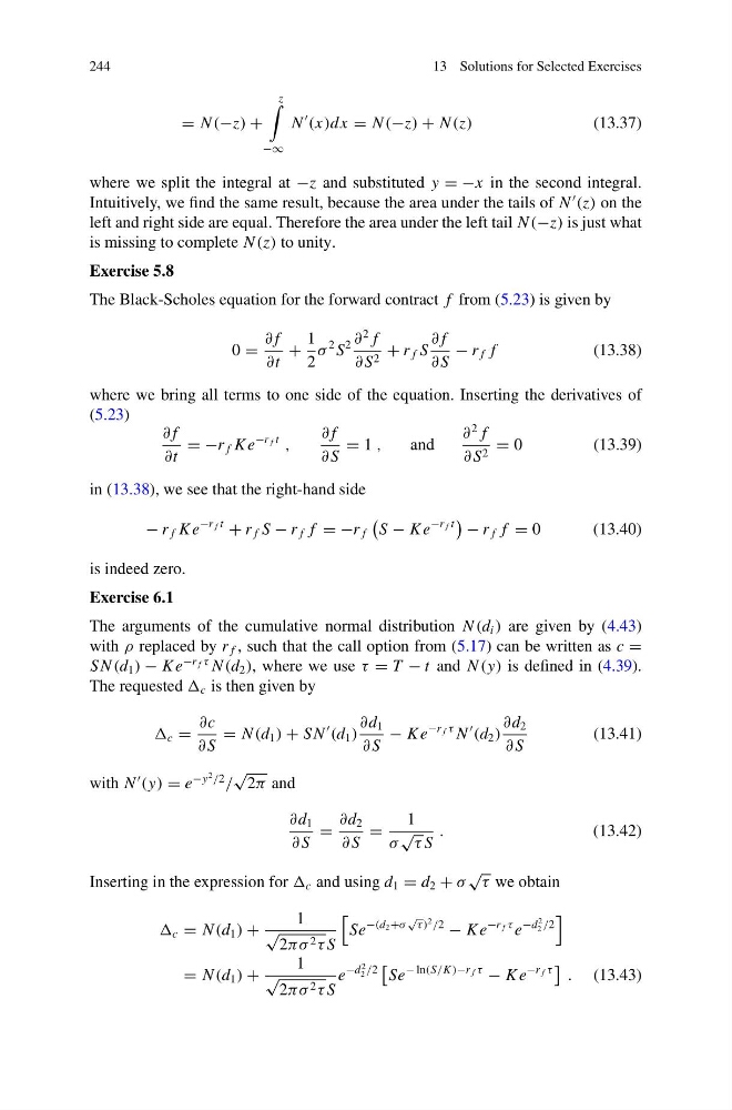
244
13 Solutions for Selected Exercises
= N (−z) +
z
−∞
N
(x)dx = N (−z) + N (z)
(13.37)
where we split the integral at −z and substituted y = −x in the second integral.
Intuitively, we find the same result, because the area under the tails of N
(z) on the
left and right side are equal. Therefore the area under the left tail N (−z) is just what
is missing to complete N (z) to unity.
Exercise 5.8
The Black-Scholes equation for the forward contract f from (5.23) is given by
0 =
∂ f
∂t
+
1
2
σ
2 S
2 ∂
2 f
∂ S 2 + r f S
∂ f
∂ S
− r f f
(13.38)
where we bring all terms to one side of the equation. Inserting the derivatives of
(5.23)
∂ f
∂t
= −r f K e
−r f t
,
∂ f
∂ S
= 1 ,
and
∂
2 f
∂ S 2 = 0
(13.39)
in (13.38), we see that the right-hand side
− r f K e
−r f t
+ r f S − r f f = −r f
S − K e
−r f t
− r f f = 0
(13.40)
is indeed zero.
Exercise 6.1
The arguments of the cumulative normal distribution N (d i ) are given by (4.43)
with ρ replaced by r f , such that the call option from (5.17) can be written as c =
S N (d 1 ) − K e
−r f τ N (d 2 ), where we use τ = T − t and N (y) is defined in (4.39).
The requested c is then given by
c =
∂c
∂ S
= N (d 1 ) + S N
(d 1 )
∂d 1
∂ S
− K e
−r f τ N
(d 2 )
∂d 2
∂ S
(13.41)
with N
(y) = e
−y
2 /2
/
√
2π and
∂d 1
∂ S
=
∂d 2
∂ S
=
1
σ
√ τ S
.
(13.42)
Inserting in the expression for c and using d 1 = d 2 + σ
√
τ we obtain
c = N (d 1 ) +
1
√
2πσ 2 τ S
Se
−(d 2 +σ
√
τ )
2 /2
− K e
−r f τ e
−d
2
2 /2
= N (d 1 ) +
1
√
2πσ 2 τ S
e
−d
2
2 /2
Se
− ln(S/K )−r f τ
− K e
−r f τ
. (13.43)