

13 Solutions for Selected Exercises
237
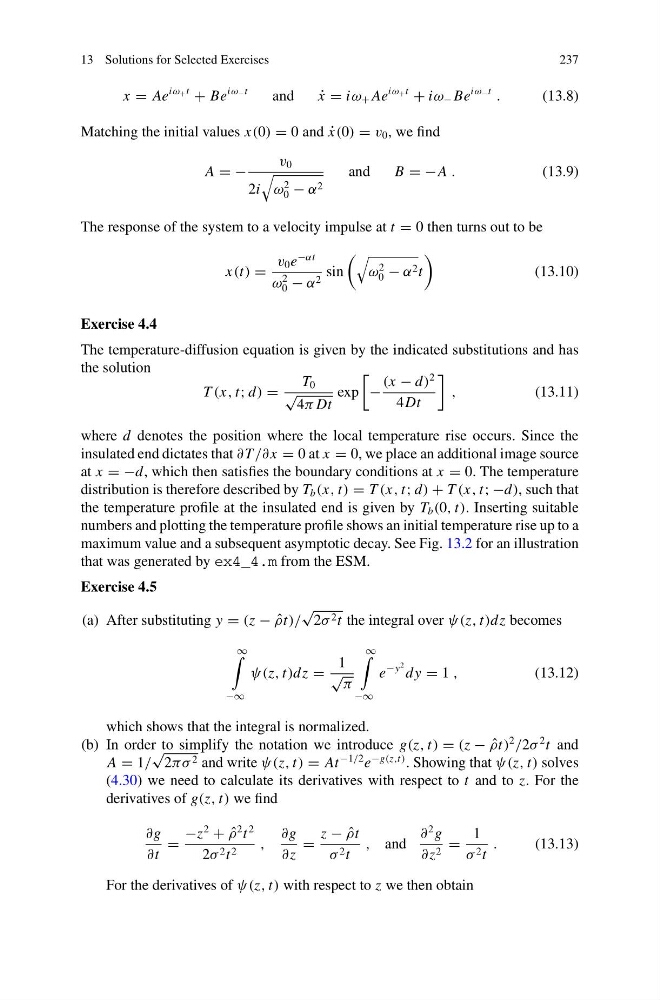
x = Ae
iω + t
+ Be
iω − t
and
˙
x = iω + Ae
iω + t
+ iω − Be
iω − t
.
(13.8)
Matching the initial values x(0) = 0 and ˙
x(0) = v 0 , we find
A = −
v 0
2i
ω
2
0 − α 2
and
B = −A .
(13.9)
The response of the system to a velocity impulse at t = 0 then turns out to be
x(t) =
v 0 e
−αt
ω
2
0 − α 2 sin
ω
2
0 − α 2 t
(13.10)
Exercise 4.4
The temperature-diffusion equation is given by the indicated substitutions and has
the solution
T (x, t; d) =
T 0
√
4π Dt
exp
−
(x − d)
2
4Dt
,
(13.11)
where d denotes the position where the local temperature rise occurs. Since the
insulated end dictates that ∂ T /∂ x = 0 at x = 0, we place an additional image source
at x = −d, which then satisfies the boundary conditions at x = 0. The temperature
distribution is therefore described by T b (x, t) = T (x, t; d) + T (x, t; −d), such that
the temperature profile at the insulated end is given by T b (0, t). Inserting suitable
numbers and plotting the temperature profile shows an initial temperature rise up to a
maximum value and a subsequent asymptotic decay. See Fig. 13.2 for an illustration
that was generated by ex4_4.m from the ESM.
Exercise 4.5
(a) After substituting y = (z − ˆ
ρt)/
√
2σ 2 t the integral over ψ(z, t)dz becomes
∞
−∞
ψ(z, t)dz =
1
√ π
∞
−∞
e
−y
2 dy = 1 ,
(13.12)
which shows that the integral is normalized.
(b) In order to simplify the notation we introduce g(z, t) = (z − ˆ
ρt)
2
/2σ
2 t and
A = 1/
√
2πσ 2 and write ψ(z, t) = At
−1/2 e
−g(z,t) . Showing that ψ(z, t) solves
(4.30) we need to calculate its derivatives with respect to t and to z. For the
derivatives of g(z, t) we find
∂g
∂t
=
−z
2
+ ˆ
ρ
2 t
2
2σ 2 t 2
,
∂g
∂z
=
z − ˆ
ρt
σ 2 t
, and
∂
2 g
∂z 2 =
1
σ 2 t
.
(13.13)
For the derivatives of ψ(z, t) with respect to z we then obtain
237
x = Ae
iω + t
+ Be
iω − t
and
˙
x = iω + Ae
iω + t
+ iω − Be
iω − t
.
(13.8)
Matching the initial values x(0) = 0 and ˙
x(0) = v 0 , we find
A = −
v 0
2i
ω
2
0 − α 2
and
B = −A .
(13.9)
The response of the system to a velocity impulse at t = 0 then turns out to be
x(t) =
v 0 e
−αt
ω
2
0 − α 2 sin
ω
2
0 − α 2 t
(13.10)
Exercise 4.4
The temperature-diffusion equation is given by the indicated substitutions and has
the solution
T (x, t; d) =
T 0
√
4π Dt
exp
−
(x − d)
2
4Dt
,
(13.11)
where d denotes the position where the local temperature rise occurs. Since the
insulated end dictates that ∂ T /∂ x = 0 at x = 0, we place an additional image source
at x = −d, which then satisfies the boundary conditions at x = 0. The temperature
distribution is therefore described by T b (x, t) = T (x, t; d) + T (x, t; −d), such that
the temperature profile at the insulated end is given by T b (0, t). Inserting suitable
numbers and plotting the temperature profile shows an initial temperature rise up to a
maximum value and a subsequent asymptotic decay. See Fig. 13.2 for an illustration
that was generated by ex4_4.m from the ESM.
Exercise 4.5
(a) After substituting y = (z − ˆ
ρt)/
√
2σ 2 t the integral over ψ(z, t)dz becomes
∞
−∞
ψ(z, t)dz =
1
√ π
∞
−∞
e
−y
2 dy = 1 ,
(13.12)
which shows that the integral is normalized.
(b) In order to simplify the notation we introduce g(z, t) = (z − ˆ
ρt)
2
/2σ
2 t and
A = 1/
√
2πσ 2 and write ψ(z, t) = At
−1/2 e
−g(z,t) . Showing that ψ(z, t) solves
(4.30) we need to calculate its derivatives with respect to t and to z. For the
derivatives of g(z, t) we find
∂g
∂t
=
−z
2
+ ˆ
ρ
2 t
2
2σ 2 t 2
,
∂g
∂z
=
z − ˆ
ρt
σ 2 t
, and
∂
2 g
∂z 2 =
1
σ 2 t
.
(13.13)
For the derivatives of ψ(z, t) with respect to z we then obtain