

234
13 Solutions for Selected Exercises
“not having” corresponds to “short”. One might hypothesize that the origin of this
nomenclature comes from medieval times, when debt was recorded with tally sticks.
These are specially marked pieces of wood that were broken in two. The shorter
piece was given to the borrower and the longer piece to the lender as a record of the
transaction.
Exercise 3.1
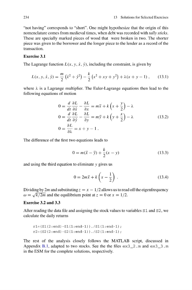
The Lagrange function L(x, y, ˙
x, ˙
y), including the constraint, is given by
L(x, y, ˙
x, ˙
y) =
m
2
˙
x
2
+ ˙
y
2
−
k
2
x
2
+ x y + y
2
+ λ(x + y − 1) ,
(13.1)
where λ is a Lagrange multiplier. The Euler-Lagrange equations then lead to the
following equations of motion
0 =
d
dt
∂ L
∂ ˙
x
−
∂ L
∂ x
= m ¨
x + k
x +
y
2
− λ
0 =
d
dt
∂ L
∂ ˙
y
−
∂ L
∂ y
= m ¨
y + k
y +
x
2
− λ
(13.2)
0 =
∂ L
∂λ
= x + y − 1 .
The difference of the first two equations leads to
0 = m( ¨
x − ¨
y) +
k
2
(x − y)
(13.3)
and using the third equation to eliminate y gives us
0 = 2m ¨
x + k
x −
1
2
.
(13.4)
Dividing by 2m and substituting z = x − 1/2 allows us to read off the eigenfrequency
ω =
√
k/2m and the equilibrium point at z = 0 or x = 1/2.
Exercise 3.2 and 3.3
After reading the data file and assigning the stock values to variables S1 and S2, we
calculate the daily returns
r1=(S1(2:end)-S1(1:end-1))./S1(1:end-1);
r2=(S2(2:end)-S2(1:end-1))./S2(1:end-1);
The rest of the analysis closely follows the MATLAB script, discussed in
Appendix B.1, adapted to two stocks. See the the files ex3_2.m and ex3_3.m
in the ESM for the complete solutions, respectively.
13 Solutions for Selected Exercises
“not having” corresponds to “short”. One might hypothesize that the origin of this
nomenclature comes from medieval times, when debt was recorded with tally sticks.
These are specially marked pieces of wood that were broken in two. The shorter
piece was given to the borrower and the longer piece to the lender as a record of the
transaction.
Exercise 3.1
The Lagrange function L(x, y, ˙
x, ˙
y), including the constraint, is given by
L(x, y, ˙
x, ˙
y) =
m
2
˙
x
2
+ ˙
y
2
−
k
2
x
2
+ x y + y
2
+ λ(x + y − 1) ,
(13.1)
where λ is a Lagrange multiplier. The Euler-Lagrange equations then lead to the
following equations of motion
0 =
d
dt
∂ L
∂ ˙
x
−
∂ L
∂ x
= m ¨
x + k
x +
y
2
− λ
0 =
d
dt
∂ L
∂ ˙
y
−
∂ L
∂ y
= m ¨
y + k
y +
x
2
− λ
(13.2)
0 =
∂ L
∂λ
= x + y − 1 .
The difference of the first two equations leads to
0 = m( ¨
x − ¨
y) +
k
2
(x − y)
(13.3)
and using the third equation to eliminate y gives us
0 = 2m ¨
x + k
x −
1
2
.
(13.4)
Dividing by 2m and substituting z = x − 1/2 allows us to read off the eigenfrequency
ω =
√
k/2m and the equilibrium point at z = 0 or x = 1/2.
Exercise 3.2 and 3.3
After reading the data file and assigning the stock values to variables S1 and S2, we
calculate the daily returns
r1=(S1(2:end)-S1(1:end-1))./S1(1:end-1);
r2=(S2(2:end)-S2(1:end-1))./S2(1:end-1);
The rest of the analysis closely follows the MATLAB script, discussed in
Appendix B.1, adapted to two stocks. See the the files ex3_2.m and ex3_3.m
in the ESM for the complete solutions, respectively.