

186
11 Optimal Control Theory
neous equation can be found by the Ansatz z p (t) = g(t)e
−αt which leads to g(t) =
−(c 1 /α
2
)e
αt
− (1/2α)(c 2 − c 1 /α)e
2αt
, such that we find for x 2 (t) = z h (t) + z p (t),
or
x 2 (t) = c 3 e
−αt
−
c 1
α 2 −
1
2α
c 2 −
c 1
α
e
αt
.
(11.46)
Using this expression allows us to integrate the third equation and determine x 1
x 1 (t) = c 4 −
c 3
α
e
−αt
−
c 1
α 2 t −
1
2α 2
c 2 −
c 1
α
e
αt
(11.47)
with a fourth integration constant c 4 . The boundary conditions for t = 0, inserted
into the equations for x 1 (t) and x 2 (t), lead to
0 = c 4 −
c 3
α
−
1
2α
c 2 −
c 1
α
and 0 = c 3 −
c 1
α 2 −
1
2α
c 2 −
c 1
α
, (11.48)
which allows us to solve for c 1 = 2α
2 c 3 − α
3 c 4 through c 3 and c 4 and likewise
for c 2 = α
2 c 4 . With these simplifications the boundary conditions for t = T can be
written as
L = c 4
1 + αT − e
αT
+ c 3
e
αT
− e
−αT
− 2αT
α
0 = c 4
α − αe
αT
+ c 3
e
αT
+ e
−αT
− 2
.
(11.49)
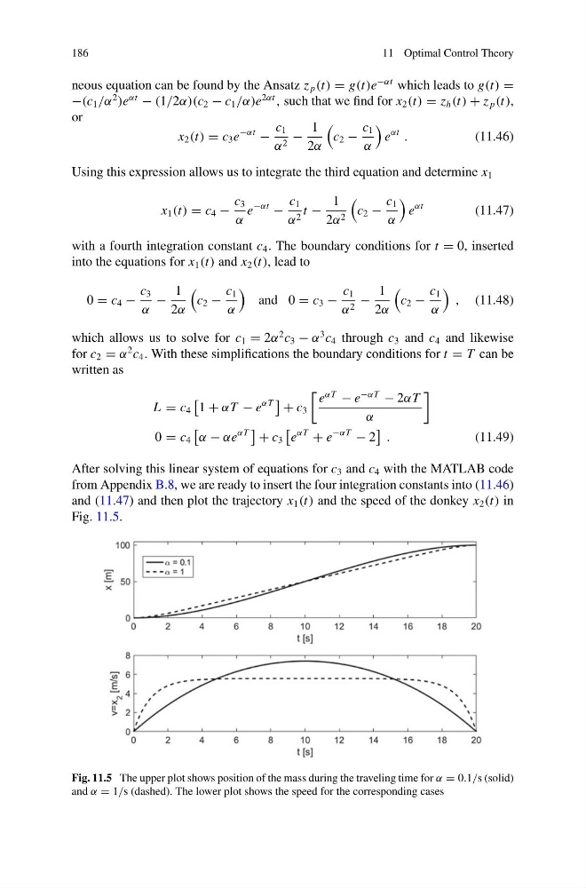
After solving this linear system of equations for c 3 and c 4 with the MATLAB code
from Appendix B.8, we are ready to insert the four integration constants into (11.46)
and (11.47) and then plot the trajectory x 1 (t) and the speed of the donkey x 2 (t) in
Fig. 11.5.
Fig. 11.5 The upper plot shows position of the mass during the traveling time for α = 0.1/s (solid)
and α = 1/s (dashed). The lower plot shows the speed for the corresponding cases
11 Optimal Control Theory
neous equation can be found by the Ansatz z p (t) = g(t)e
−αt which leads to g(t) =
−(c 1 /α
2
)e
αt
− (1/2α)(c 2 − c 1 /α)e
2αt
, such that we find for x 2 (t) = z h (t) + z p (t),
or
x 2 (t) = c 3 e
−αt
−
c 1
α 2 −
1
2α
c 2 −
c 1
α
e
αt
.
(11.46)
Using this expression allows us to integrate the third equation and determine x 1
x 1 (t) = c 4 −
c 3
α
e
−αt
−
c 1
α 2 t −
1
2α 2
c 2 −
c 1
α
e
αt
(11.47)
with a fourth integration constant c 4 . The boundary conditions for t = 0, inserted
into the equations for x 1 (t) and x 2 (t), lead to
0 = c 4 −
c 3
α
−
1
2α
c 2 −
c 1
α
and 0 = c 3 −
c 1
α 2 −
1
2α
c 2 −
c 1
α
, (11.48)
which allows us to solve for c 1 = 2α
2 c 3 − α
3 c 4 through c 3 and c 4 and likewise
for c 2 = α
2 c 4 . With these simplifications the boundary conditions for t = T can be
written as
L = c 4
1 + αT − e
αT
+ c 3
e
αT
− e
−αT
− 2αT
α
0 = c 4
α − αe
αT
+ c 3
e
αT
+ e
−αT
− 2
.
(11.49)
After solving this linear system of equations for c 3 and c 4 with the MATLAB code
from Appendix B.8, we are ready to insert the four integration constants into (11.46)
and (11.47) and then plot the trajectory x 1 (t) and the speed of the donkey x 2 (t) in
Fig. 11.5.
Fig. 11.5 The upper plot shows position of the mass during the traveling time for α = 0.1/s (solid)
and α = 1/s (dashed). The lower plot shows the speed for the corresponding cases