

11.5 Donkey Revisited
185
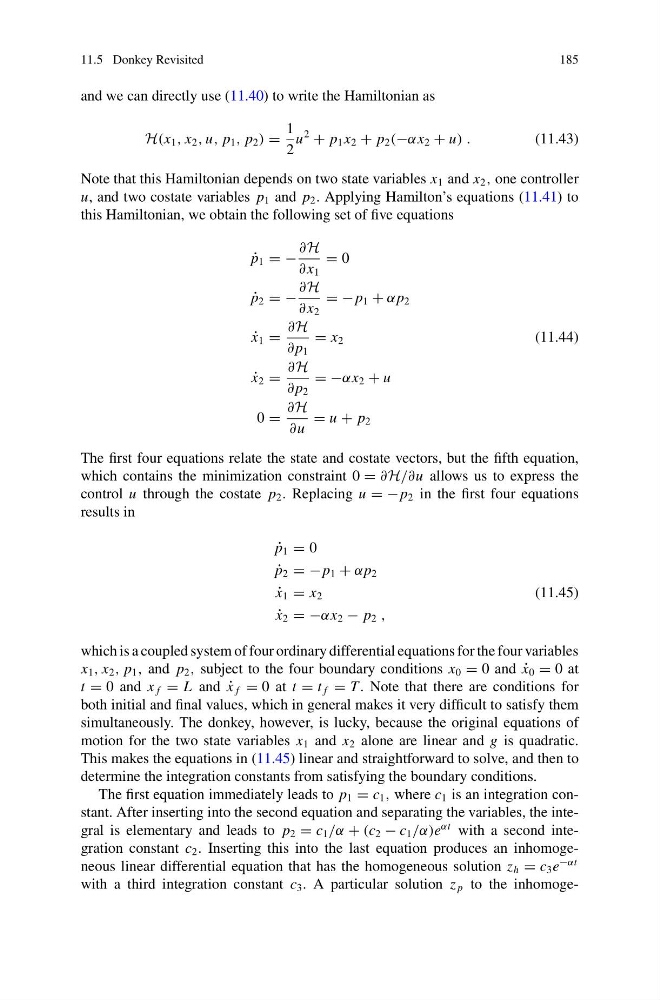
and we can directly use (11.40) to write the Hamiltonian as
H(x 1 , x 2 , u, p 1 , p 2 ) =
1
2
u
2
+ p 1 x 2 + p 2 (−αx 2 + u) .
(11.43)
Note that this Hamiltonian depends on two state variables x 1 and x 2 , one controller
u, and two costate variables p 1 and p 2 . Applying Hamilton’s equations (11.41) to
this Hamiltonian, we obtain the following set of five equations
˙
p 1 = −
∂H
∂ x 1
= 0
˙
p 2 = −
∂H
∂ x 2
= −p 1 + αp 2
˙
x 1 =
∂H
∂ p 1
= x 2
(11.44)
˙
x 2 =
∂H
∂ p 2
= −αx 2 + u
0 =
∂H
∂u
= u + p 2
The first four equations relate the state and costate vectors, but the fifth equation,
which contains the minimization constraint 0 = ∂H/∂u allows us to express the
control u through the costate p 2 . Replacing u = −p 2 in the first four equations
results in
˙
p 1 = 0
˙
p 2 = −p 1 + αp 2
˙
x 1 = x 2
(11.45)
˙
x 2 = −αx 2 − p 2 ,
which is a coupled system of four ordinary differential equations for the four variables
x 1 , x 2 , p 1 , and p 2 , subject to the four boundary conditions x 0 = 0 and ˙
x 0 = 0 at
t = 0 and x f = L and ˙
x f = 0 at t = t f = T. Note that there are conditions for
both initial and final values, which in general makes it very difficult to satisfy them
simultaneously. The donkey, however, is lucky, because the original equations of
motion for the two state variables x 1 and x 2 alone are linear and g is quadratic.
This makes the equations in (11.45) linear and straightforward to solve, and then to
determine the integration constants from satisfying the boundary conditions.
The first equation immediately leads to p 1 = c 1 , where c 1 is an integration constant. After inserting into the second equation and separating the variables, the integral is elementary and leads to p 2 = c 1 /α + (c 2 − c 1 /α)e
αt with a second integration constant c 2 . Inserting this into the last equation produces an inhomogeneous linear differential equation that has the homogeneous solution z h = c 3 e
−αt
with a third integration constant c 3 . A particular solution z p to the inhomoge-
185
and we can directly use (11.40) to write the Hamiltonian as
H(x 1 , x 2 , u, p 1 , p 2 ) =
1
2
u
2
+ p 1 x 2 + p 2 (−αx 2 + u) .
(11.43)
Note that this Hamiltonian depends on two state variables x 1 and x 2 , one controller
u, and two costate variables p 1 and p 2 . Applying Hamilton’s equations (11.41) to
this Hamiltonian, we obtain the following set of five equations
˙
p 1 = −
∂H
∂ x 1
= 0
˙
p 2 = −
∂H
∂ x 2
= −p 1 + αp 2
˙
x 1 =
∂H
∂ p 1
= x 2
(11.44)
˙
x 2 =
∂H
∂ p 2
= −αx 2 + u
0 =
∂H
∂u
= u + p 2
The first four equations relate the state and costate vectors, but the fifth equation,
which contains the minimization constraint 0 = ∂H/∂u allows us to express the
control u through the costate p 2 . Replacing u = −p 2 in the first four equations
results in
˙
p 1 = 0
˙
p 2 = −p 1 + αp 2
˙
x 1 = x 2
(11.45)
˙
x 2 = −αx 2 − p 2 ,
which is a coupled system of four ordinary differential equations for the four variables
x 1 , x 2 , p 1 , and p 2 , subject to the four boundary conditions x 0 = 0 and ˙
x 0 = 0 at
t = 0 and x f = L and ˙
x f = 0 at t = t f = T. Note that there are conditions for
both initial and final values, which in general makes it very difficult to satisfy them
simultaneously. The donkey, however, is lucky, because the original equations of
motion for the two state variables x 1 and x 2 alone are linear and g is quadratic.
This makes the equations in (11.45) linear and straightforward to solve, and then to
determine the integration constants from satisfying the boundary conditions.
The first equation immediately leads to p 1 = c 1 , where c 1 is an integration constant. After inserting into the second equation and separating the variables, the integral is elementary and leads to p 2 = c 1 /α + (c 2 − c 1 /α)e
αt with a second integration constant c 2 . Inserting this into the last equation produces an inhomogeneous linear differential equation that has the homogeneous solution z h = c 3 e
−αt
with a third integration constant c 3 . A particular solution z p to the inhomoge-