

180
11 Optimal Control Theory
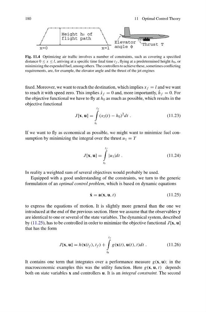
Fig. 11.4 Optimizing air traffic involves a number of constraints, such as covering a specified
distance 0 ≤ x ≤ l, arriving at a specific time final time t f , flying at a predetermined height h 0 , or
minimizing the expended fuel, among others. The controllers to achieve these, sometimes conflicting
requirements, are, for example, the elevator angle and the thrust of the jet engines
fixed. Moreover, we want to reach the destination, which implies x f = l and we want
to reach it with speed zero. This implies ˙
x f = 0 and, more importantly, ˙
h f = 0. For
the objective functional we have to fly at h 0 as much as possible, which results in the
objective functional
J [x, u] =
t f
t 0
(x 2 (t) − h 0 )
2 dt .
(11.23)
If we want to fly as economical as possible, we might want to minimize fuel consumption by minimizing the integral over the thrust u 1 = T
J [x, u] =
t f
t 0
|u 1 |dt .
(11.24)
In reality a weighted sum of several objectives would probably be used.
Equipped with a good understanding of the constraints, we turn to the generic
formulation of an optimal control problem, which is based on dynamic equations
˙
x = a(x, u, t)
(11.25)
to express the equations of motion. It is slightly more general than the one we
introduced at the end of the previous section. Here we assume that the observables y
are identical to one or several of the state variables. The dynamical system, described
by (11.25), has to be controlled in order to minimize the objective functional J [x, u]
that has the form
J [x, u] = h(x(t f ), t f ) +
t f
t 0
g(x(t), u(t), t)dt .
(11.26)
It contains one term that integrates over a performance measure g(x, u); in the
macroeconomic examples this was the utility function. Here g(x, u, t) depends
both on state variables x and controllers u. It is an integral constraint. The second
11 Optimal Control Theory
Fig. 11.4 Optimizing air traffic involves a number of constraints, such as covering a specified
distance 0 ≤ x ≤ l, arriving at a specific time final time t f , flying at a predetermined height h 0 , or
minimizing the expended fuel, among others. The controllers to achieve these, sometimes conflicting
requirements, are, for example, the elevator angle and the thrust of the jet engines
fixed. Moreover, we want to reach the destination, which implies x f = l and we want
to reach it with speed zero. This implies ˙
x f = 0 and, more importantly, ˙
h f = 0. For
the objective functional we have to fly at h 0 as much as possible, which results in the
objective functional
J [x, u] =
t f
t 0
(x 2 (t) − h 0 )
2 dt .
(11.23)
If we want to fly as economical as possible, we might want to minimize fuel consumption by minimizing the integral over the thrust u 1 = T
J [x, u] =
t f
t 0
|u 1 |dt .
(11.24)
In reality a weighted sum of several objectives would probably be used.
Equipped with a good understanding of the constraints, we turn to the generic
formulation of an optimal control problem, which is based on dynamic equations
˙
x = a(x, u, t)
(11.25)
to express the equations of motion. It is slightly more general than the one we
introduced at the end of the previous section. Here we assume that the observables y
are identical to one or several of the state variables. The dynamical system, described
by (11.25), has to be controlled in order to minimize the objective functional J [x, u]
that has the form
J [x, u] = h(x(t f ), t f ) +
t f
t 0
g(x(t), u(t), t)dt .
(11.26)
It contains one term that integrates over a performance measure g(x, u); in the
macroeconomic examples this was the utility function. Here g(x, u, t) depends
both on state variables x and controllers u. It is an integral constraint. The second