

11.2 Control and Feedback
179
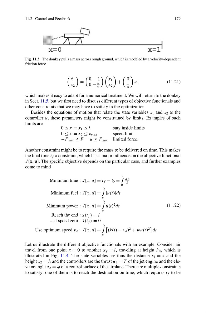
Fig. 11.3 The donkey pulls a mass across rough ground, which is modeled by a velocity-dependent
friction force
˙
x 1
˙
x 2
=
0 1
0 −
α
m
x 1
x 2
+
0
1
m
u ,
(11.21)
which makes it easy to adapt for a numerical treatment. We will return to the donkey
in Sect. 11.5, but we first need to discuss different types of objective functionals and
other constraints that we may have to satisfy in the optimization.
Besides the equations of motion that relate the state variables x 1 and x 2 to the
controller u, these parameters might be constrained by limits. Examples of such
limits are
0 ≤ x = x 1 ≤ l
stay inside limits
0 ≤ ˙
x = x 2 ≤ v max
speed limit
−F max ≤ F = u ≤ F max limited force.
Another constraint might be to require the mass to be delivered on time. This makes
the final time t f a constraint, which has a major influence on the objective functional
J [x, u]. The specific objective depends on the particular case, and further examples
come to mind
Minimum time : J [x, u] = t f − t 0 =
l
0
dx
˙
x
Minimum fuel : J [x, u] =
t f
t 0
|u(t)|dt
Minimum power : J [x, u] =
t f
t 0
u(t)
2 dt
Reach the end : x(t f ) = l
...at speed zero : ˙
x(t f ) = 0
Use optimum speed v d : J [x, u] =
t f
t 0
( ˙
x(t) − v d )
2
+ wu(t)
2
dt
(11.22)
Let us illustrate the different objective functionals with an example. Consider air
travel from one point x = 0 to another x f = l, traveling at height h 0 , which is
illustrated in Fig. 11.4. The state variables are thus the distance x 1 = x and the
height x 2 = h and the controllers are the thrust u 1 = T of the jet engine and the elevator angle u 2 = φ of a control surface of the airplane. There are multiple constraints
to satisfy: one of them is to reach the destination on time, which requires t f to be
179
Fig. 11.3 The donkey pulls a mass across rough ground, which is modeled by a velocity-dependent
friction force
˙
x 1
˙
x 2
=
0 1
0 −
α
m
x 1
x 2
+
0
1
m
u ,
(11.21)
which makes it easy to adapt for a numerical treatment. We will return to the donkey
in Sect. 11.5, but we first need to discuss different types of objective functionals and
other constraints that we may have to satisfy in the optimization.
Besides the equations of motion that relate the state variables x 1 and x 2 to the
controller u, these parameters might be constrained by limits. Examples of such
limits are
0 ≤ x = x 1 ≤ l
stay inside limits
0 ≤ ˙
x = x 2 ≤ v max
speed limit
−F max ≤ F = u ≤ F max limited force.
Another constraint might be to require the mass to be delivered on time. This makes
the final time t f a constraint, which has a major influence on the objective functional
J [x, u]. The specific objective depends on the particular case, and further examples
come to mind
Minimum time : J [x, u] = t f − t 0 =
l
0
dx
˙
x
Minimum fuel : J [x, u] =
t f
t 0
|u(t)|dt
Minimum power : J [x, u] =
t f
t 0
u(t)
2 dt
Reach the end : x(t f ) = l
...at speed zero : ˙
x(t f ) = 0
Use optimum speed v d : J [x, u] =
t f
t 0
( ˙
x(t) − v d )
2
+ wu(t)
2
dt
(11.22)
Let us illustrate the different objective functionals with an example. Consider air
travel from one point x = 0 to another x f = l, traveling at height h 0 , which is
illustrated in Fig. 11.4. The state variables are thus the distance x 1 = x and the
height x 2 = h and the controllers are the thrust u 1 = T of the jet engine and the elevator angle u 2 = φ of a control surface of the airplane. There are multiple constraints
to satisfy: one of them is to reach the destination on time, which requires t f to be