

11.1 Macroeconomic Models
173
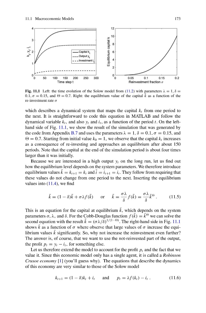
Fig. 11.1 Left: the time evolution of the Solow model from (11.2) with parameters λ = 1, δ =
0.1, σ = 0.15, and = 0.7. Right: the equilibrium value of the capital ¯
k as a function of the
re-investment rate σ
which describes a dynamical system that maps the capital k t from one period to
the next. It is straightforward to code this equation in MATLAB and follow the
dynamical variable k t , and also y t and i t , as a function of the period t. On the lefthand side of Fig. 11.1, we show the result of the simulation that was generated by
the code from Appendix B.7 and uses the parameters λ = 1, δ = 0.1, σ = 0.15, and
= 0.7. Starting from initial value k 0 = 1, we observe that the capital k t increases
as a consequence of re-investing and approaches an equilibrium after about 150
periods. Note that the capital at the end of the simulation period is about four times
larger than it was initially.
Because we are interested in a high output y t on the long run, let us find out
how the equilibrium level depends on the system parameters. We therefore introduce
equilibrium values ¯
k = k t+1 = k t and ¯
i = i t+1 = i t . They follow from requiring that
these values do not change from one period to the next. Inserting the equilibrium
values into (11.4), we find
¯
k = (1 − δ) ¯
k + σ λ f ( ¯
k)
or
¯
k =
σ λ
δ
f ( ¯
k) =
σ λ
δ
¯
k
.
(11.5)
This is an equation for the capital at equilibrium ¯
k, which depends on the system
parameters σ, λ, and δ. For the Cobb-Douglas function f ( ¯
k) = ¯
k
we can solve the
second equation with the result ¯
k = (σ λ/δ)
1/(1−) . The right-hand side in Fig. 11.1
shows ¯
k as a function of σ where observe that large values of σ increase the equilibrium values ¯
k significantly. So, why not increase the reinvestment even further?
The answer is, of course, that we want to use the not-reinvested part of the output,
the profit p t = y t − i t , for something else.
Let us therefore extend the model to account for the profit p t and the fact that we
value it. Since this economic model only has a single agent, it is called a Robinson
Crusoe economy [1] (you’ll guess why). The equations that describe the dynamics
of this economy are very similar to those of the Solow model
k t+1 = (1 − δ)k t + i t
and
p t = λ f (k t ) − i t .
(11.6)
173
Fig. 11.1 Left: the time evolution of the Solow model from (11.2) with parameters λ = 1, δ =
0.1, σ = 0.15, and = 0.7. Right: the equilibrium value of the capital ¯
k as a function of the
re-investment rate σ
which describes a dynamical system that maps the capital k t from one period to
the next. It is straightforward to code this equation in MATLAB and follow the
dynamical variable k t , and also y t and i t , as a function of the period t. On the lefthand side of Fig. 11.1, we show the result of the simulation that was generated by
the code from Appendix B.7 and uses the parameters λ = 1, δ = 0.1, σ = 0.15, and
= 0.7. Starting from initial value k 0 = 1, we observe that the capital k t increases
as a consequence of re-investing and approaches an equilibrium after about 150
periods. Note that the capital at the end of the simulation period is about four times
larger than it was initially.
Because we are interested in a high output y t on the long run, let us find out
how the equilibrium level depends on the system parameters. We therefore introduce
equilibrium values ¯
k = k t+1 = k t and ¯
i = i t+1 = i t . They follow from requiring that
these values do not change from one period to the next. Inserting the equilibrium
values into (11.4), we find
¯
k = (1 − δ) ¯
k + σ λ f ( ¯
k)
or
¯
k =
σ λ
δ
f ( ¯
k) =
σ λ
δ
¯
k
.
(11.5)
This is an equation for the capital at equilibrium ¯
k, which depends on the system
parameters σ, λ, and δ. For the Cobb-Douglas function f ( ¯
k) = ¯
k
we can solve the
second equation with the result ¯
k = (σ λ/δ)
1/(1−) . The right-hand side in Fig. 11.1
shows ¯
k as a function of σ where observe that large values of σ increase the equilibrium values ¯
k significantly. So, why not increase the reinvestment even further?
The answer is, of course, that we want to use the not-reinvested part of the output,
the profit p t = y t − i t , for something else.
Let us therefore extend the model to account for the profit p t and the fact that we
value it. Since this economic model only has a single agent, it is called a Robinson
Crusoe economy [1] (you’ll guess why). The equations that describe the dynamics
of this economy are very similar to those of the Solow model
k t+1 = (1 − δ)k t + i t
and
p t = λ f (k t ) − i t .
(11.6)