

136
9 Bubbles, Crashes, Fat Tails and Lévy-Stable Distributions
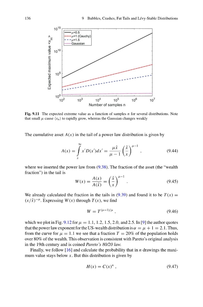
Fig. 9.11 The expected extreme value as a function of samples n for several distributions. Note
that small μ cause x n to rapidly grow, whereas the Gaussian changes weakly
The cumulative asset A(x) in the tail of a power law distribution is given by
A(x) =
∞
x
x
D(x
)dx
=
μ ˆ
x
μ − 1
ˆ
x
x
μ−1
,
(9.44)
where we inserted the power law from (9.38). The fraction of the asset (the “wealth
fraction”) in the tail is
W (x) =
A(x)
A( ˆ
x)
=
ˆ
x
x
μ−1
.
(9.45)
We already calculated the fraction in the tails in (9.39) and found it to be T (x) =
(x/ ˆ
x)
−μ . Expressing W (x) through T (x), we find
W = T
(μ−1)/μ
,
(9.46)
which we plot in Fig. 9.12 for μ = 1.1, 1.2, 1.5, 2.0, and 2.5. In [9] the author quotes
that the power law exponent for the US-wealth distribution is α = μ + 1 = 2.1. Thus,
from the curve for μ = 1.1 we see that a fraction T = 20% of the population holds
over 80% of the wealth. This observation is consistent with Pareto’s original analysis
in the 19th century and is coined Pareto’s 80/20 law.
Finally, we follow [16] and calculate the probability that in n drawings the maximum value stays below x. But this distribution is given by
H (x) = C(x)
n
,
(9.47)
9 Bubbles, Crashes, Fat Tails and Lévy-Stable Distributions
Fig. 9.11 The expected extreme value as a function of samples n for several distributions. Note
that small μ cause x n to rapidly grow, whereas the Gaussian changes weakly
The cumulative asset A(x) in the tail of a power law distribution is given by
A(x) =
∞
x
x
D(x
)dx
=
μ ˆ
x
μ − 1
ˆ
x
x
μ−1
,
(9.44)
where we inserted the power law from (9.38). The fraction of the asset (the “wealth
fraction”) in the tail is
W (x) =
A(x)
A( ˆ
x)
=
ˆ
x
x
μ−1
.
(9.45)
We already calculated the fraction in the tails in (9.39) and found it to be T (x) =
(x/ ˆ
x)
−μ . Expressing W (x) through T (x), we find
W = T
(μ−1)/μ
,
(9.46)
which we plot in Fig. 9.12 for μ = 1.1, 1.2, 1.5, 2.0, and 2.5. In [9] the author quotes
that the power law exponent for the US-wealth distribution is α = μ + 1 = 2.1. Thus,
from the curve for μ = 1.1 we see that a fraction T = 20% of the population holds
over 80% of the wealth. This observation is consistent with Pareto’s original analysis
in the 19th century and is coined Pareto’s 80/20 law.
Finally, we follow [16] and calculate the probability that in n drawings the maximum value stays below x. But this distribution is given by
H (x) = C(x)
n
,
(9.47)