

132
9 Bubbles, Crashes, Fat Tails and Lévy-Stable Distributions
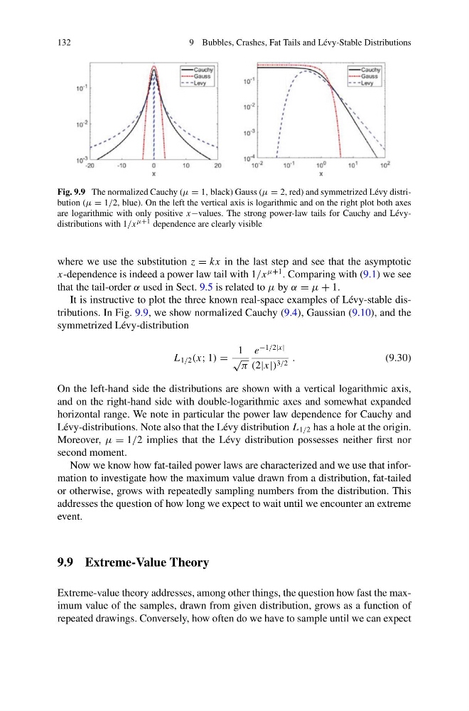
Fig. 9.9 The normalized Cauchy (μ = 1, black) Gauss (μ = 2, red) and symmetrized Lévy distribution (μ = 1/2, blue). On the left the vertical axis is logarithmic and on the right plot both axes
are logarithmic with only positive x−values. The strong power-law tails for Cauchy and Lévydistributions with 1/x μ+1 dependence are clearly visible
where we use the substitution z = kx in the last step and see that the asymptotic
x-dependence is indeed a power law tail with 1/x
μ+1
. Comparing with (9.1) we see
that the tail-order α used in Sect. 9.5 is related to μ by α = μ + 1.
It is instructive to plot the three known real-space examples of Lévy-stable distributions. In Fig. 9.9, we show normalized Cauchy (9.4), Gaussian (9.10), and the
symmetrized Lévy-distribution
L 1/2 (x; 1) =
1
√ π
e
−1/2|x|
(2|x|) 3/2 .
(9.30)
On the left-hand side the distributions are shown with a vertical logarithmic axis,
and on the right-hand side with double-logarithmic axes and somewhat expanded
horizontal range. We note in particular the power law dependence for Cauchy and
Lévy-distributions. Note also that the Lévy distribution L 1/2 has a hole at the origin.
Moreover, μ = 1/2 implies that the Lévy distribution possesses neither first nor
second moment.
Now we know how fat-tailed power laws are characterized and we use that information to investigate how the maximum value drawn from a distribution, fat-tailed
or otherwise, grows with repeatedly sampling numbers from the distribution. This
addresses the question of how long we expect to wait until we encounter an extreme
event.
9.9 Extreme-Value Theory
Extreme-value theory addresses, among other things, the question how fast the maximum value of the samples, drawn from given distribution, grows as a function of
repeated drawings. Conversely, how often do we have to sample until we can expect
9 Bubbles, Crashes, Fat Tails and Lévy-Stable Distributions
Fig. 9.9 The normalized Cauchy (μ = 1, black) Gauss (μ = 2, red) and symmetrized Lévy distribution (μ = 1/2, blue). On the left the vertical axis is logarithmic and on the right plot both axes
are logarithmic with only positive x−values. The strong power-law tails for Cauchy and Lévydistributions with 1/x μ+1 dependence are clearly visible
where we use the substitution z = kx in the last step and see that the asymptotic
x-dependence is indeed a power law tail with 1/x
μ+1
. Comparing with (9.1) we see
that the tail-order α used in Sect. 9.5 is related to μ by α = μ + 1.
It is instructive to plot the three known real-space examples of Lévy-stable distributions. In Fig. 9.9, we show normalized Cauchy (9.4), Gaussian (9.10), and the
symmetrized Lévy-distribution
L 1/2 (x; 1) =
1
√ π
e
−1/2|x|
(2|x|) 3/2 .
(9.30)
On the left-hand side the distributions are shown with a vertical logarithmic axis,
and on the right-hand side with double-logarithmic axes and somewhat expanded
horizontal range. We note in particular the power law dependence for Cauchy and
Lévy-distributions. Note also that the Lévy distribution L 1/2 has a hole at the origin.
Moreover, μ = 1/2 implies that the Lévy distribution possesses neither first nor
second moment.
Now we know how fat-tailed power laws are characterized and we use that information to investigate how the maximum value drawn from a distribution, fat-tailed
or otherwise, grows with repeatedly sampling numbers from the distribution. This
addresses the question of how long we expect to wait until we encounter an extreme
event.
9.9 Extreme-Value Theory
Extreme-value theory addresses, among other things, the question how fast the maximum value of the samples, drawn from given distribution, grows as a function of
repeated drawings. Conversely, how often do we have to sample until we can expect