

9.8 Lévy-Stable Distributions
131
˜
L μ (k; 1) = e
−a|k|
μ
with 0 < μ < 2
(9.26)
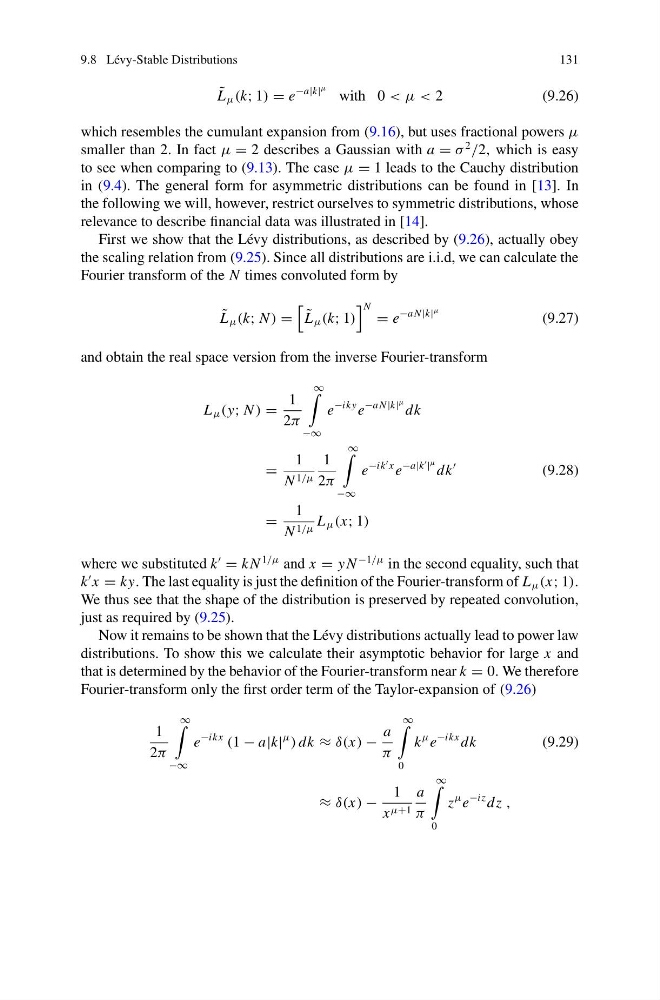
which resembles the cumulant expansion from (9.16), but uses fractional powers μ
smaller than 2. In fact μ = 2 describes a Gaussian with a = σ
2
/2, which is easy
to see when comparing to (9.13). The case μ = 1 leads to the Cauchy distribution
in (9.4). The general form for asymmetric distributions can be found in [13]. In
the following we will, however, restrict ourselves to symmetric distributions, whose
relevance to describe financial data was illustrated in [14].
First we show that the Lévy distributions, as described by (9.26), actually obey
the scaling relation from (9.25). Since all distributions are i.i.d, we can calculate the
Fourier transform of the N times convoluted form by
˜
L μ (k; N ) =
˜
L μ (k; 1)
N = e
−aN|k|
μ
(9.27)
and obtain the real space version from the inverse Fourier-transform
L μ (y; N ) =
1
2π
∞
−∞
e
−iky e
−aN|k|
μ dk
=
1
N 1/μ
1
2π
∞
−∞
e
−ik
x e
−a|k
|
μ dk
(9.28)
=
1
N 1/μ L μ (x; 1)
where we substituted k
= k N
1/μ and x = y N
−1/μ in the second equality, such that
k
x = ky. The last equality is just the definition of the Fourier-transform of L μ (x; 1).
We thus see that the shape of the distribution is preserved by repeated convolution,
just as required by (9.25).
Now it remains to be shown that the Lévy distributions actually lead to power law
distributions. To show this we calculate their asymptotic behavior for large x and
that is determined by the behavior of the Fourier-transform near k = 0. We therefore
Fourier-transform only the first order term of the Taylor-expansion of (9.26)
1
2π
∞
−∞
e
−ikx
(1 − a|k|
μ
) dk ≈ δ(x) −
a
π
∞
0
k
μ e
−ikx dk
(9.29)
≈ δ(x) −
1
x μ+1
a
π
∞
0
z
μ e
−iz dz ,
131
˜
L μ (k; 1) = e
−a|k|
μ
with 0 < μ < 2
(9.26)
which resembles the cumulant expansion from (9.16), but uses fractional powers μ
smaller than 2. In fact μ = 2 describes a Gaussian with a = σ
2
/2, which is easy
to see when comparing to (9.13). The case μ = 1 leads to the Cauchy distribution
in (9.4). The general form for asymmetric distributions can be found in [13]. In
the following we will, however, restrict ourselves to symmetric distributions, whose
relevance to describe financial data was illustrated in [14].
First we show that the Lévy distributions, as described by (9.26), actually obey
the scaling relation from (9.25). Since all distributions are i.i.d, we can calculate the
Fourier transform of the N times convoluted form by
˜
L μ (k; N ) =
˜
L μ (k; 1)
N = e
−aN|k|
μ
(9.27)
and obtain the real space version from the inverse Fourier-transform
L μ (y; N ) =
1
2π
∞
−∞
e
−iky e
−aN|k|
μ dk
=
1
N 1/μ
1
2π
∞
−∞
e
−ik
x e
−a|k
|
μ dk
(9.28)
=
1
N 1/μ L μ (x; 1)
where we substituted k
= k N
1/μ and x = y N
−1/μ in the second equality, such that
k
x = ky. The last equality is just the definition of the Fourier-transform of L μ (x; 1).
We thus see that the shape of the distribution is preserved by repeated convolution,
just as required by (9.25).
Now it remains to be shown that the Lévy distributions actually lead to power law
distributions. To show this we calculate their asymptotic behavior for large x and
that is determined by the behavior of the Fourier-transform near k = 0. We therefore
Fourier-transform only the first order term of the Taylor-expansion of (9.26)
1
2π
∞
−∞
e
−ikx
(1 − a|k|
μ
) dk ≈ δ(x) −
a
π
∞
0
k
μ e
−ikx dk
(9.29)
≈ δ(x) −
1
x μ+1
a
π
∞
0
z
μ e
−iz dz ,