

104
8 Time Series
y m+n =
⎛
⎝ 1 −
∞
j=n+1
π j ˆ
L
j
⎞
⎠ ε m .
(8.29)
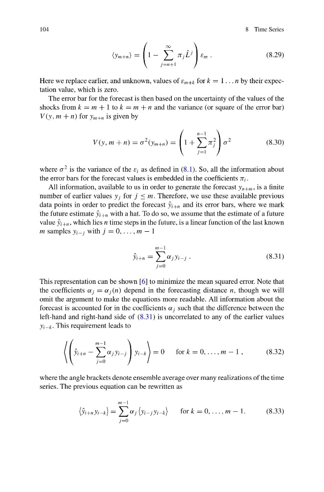
Here we replace earlier, and unknown, values of ε m+k for k = 1 . . . n by their expectation value, which is zero.
The error bar for the forecast is then based on the uncertainty of the values of the
shocks from k = m + 1 to k = m + n and the variance (or square of the error bar)
V (y, m + n) for y m+n is given by
V (y, m + n) = σ
2
(y m+n ) =
⎛
⎝ 1 +
n−1
j=1
π
2
j
⎞
⎠ σ
2
(8.30)
where σ
2 is the variance of the ε i as defined in (8.1). So, all the information about
the error bars for the forecast values is embedded in the coefficients π i .
All information, available to us in order to generate the forecast y n+m , is a finite
number of earlier values y j for j ≤ m. Therefore, we use these available previous
data points in order to predict the forecast ˆ
y i+n and its error bars, where we mark
the future estimate ˆ
y i+n with a hat. To do so, we assume that the estimate of a future
value ˆ
y i+n , which lies n time steps in the future, is a linear function of the last known
m samples y i− j with j = 0, . . . , m − 1
ˆ
y i+n =
m−1
j=0
α j y i− j .
(8.31)
This representation can be shown [6] to minimize the mean squared error. Note that
the coefficients α j = α j (n) depend in the forecasting distance n, though we will
omit the argument to make the equations more readable. All information about the
forecast is accounted for in the coefficients α j such that the difference between the
left-hand and right-hand side of (8.31) is uncorrelated to any of the earlier values
y i−k . This requirement leads to
⎛
⎝ ˆ
y i+n −
m−1
j=0
α j y i− j
⎞
⎠ y i−k
= 0
for k = 0, . . . , m − 1 ,
(8.32)
where the angle brackets denote ensemble average over many realizations of the time
series. The previous equation can be rewritten as
ˆ
y i+n y i−k
=
m−1
j=0
α j
y i− j y i−k
for k = 0, . . . , m − 1.
(8.33)
8 Time Series
y m+n =
⎛
⎝ 1 −
∞
j=n+1
π j ˆ
L
j
⎞
⎠ ε m .
(8.29)
Here we replace earlier, and unknown, values of ε m+k for k = 1 . . . n by their expectation value, which is zero.
The error bar for the forecast is then based on the uncertainty of the values of the
shocks from k = m + 1 to k = m + n and the variance (or square of the error bar)
V (y, m + n) for y m+n is given by
V (y, m + n) = σ
2
(y m+n ) =
⎛
⎝ 1 +
n−1
j=1
π
2
j
⎞
⎠ σ
2
(8.30)
where σ
2 is the variance of the ε i as defined in (8.1). So, all the information about
the error bars for the forecast values is embedded in the coefficients π i .
All information, available to us in order to generate the forecast y n+m , is a finite
number of earlier values y j for j ≤ m. Therefore, we use these available previous
data points in order to predict the forecast ˆ
y i+n and its error bars, where we mark
the future estimate ˆ
y i+n with a hat. To do so, we assume that the estimate of a future
value ˆ
y i+n , which lies n time steps in the future, is a linear function of the last known
m samples y i− j with j = 0, . . . , m − 1
ˆ
y i+n =
m−1
j=0
α j y i− j .
(8.31)
This representation can be shown [6] to minimize the mean squared error. Note that
the coefficients α j = α j (n) depend in the forecasting distance n, though we will
omit the argument to make the equations more readable. All information about the
forecast is accounted for in the coefficients α j such that the difference between the
left-hand and right-hand side of (8.31) is uncorrelated to any of the earlier values
y i−k . This requirement leads to
⎛
⎝ ˆ
y i+n −
m−1
j=0
α j y i− j
⎞
⎠ y i−k
= 0
for k = 0, . . . , m − 1 ,
(8.32)
where the angle brackets denote ensemble average over many realizations of the time
series. The previous equation can be rewritten as
ˆ
y i+n y i−k
=
m−1
j=0
α j
y i− j y i−k
for k = 0, . . . , m − 1.
(8.33)