

102
8 Time Series
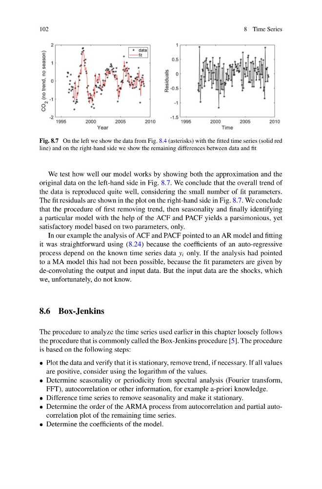
Fig. 8.7 On the left we show the data from Fig. 8.4 (asterisks) with the fitted time series (solid red
line) and on the right-hand side we show the remaining differences between data and fit
We test how well our model works by showing both the approximation and the
original data on the left-hand side in Fig. 8.7. We conclude that the overall trend of
the data is reproduced quite well, considering the small number of fit parameters.
The fit residuals are shown in the plot on the right-hand side in Fig. 8.7. We conclude
that the procedure of first removing trend, then seasonality and finally identifying
a particular model with the help of the ACF and PACF yields a parsimonious, yet
satisfactory model based on two parameters, only.
In our example the analysis of ACF and PACF pointed to an AR model and fitting
it was straightforward using (8.24) because the coefficients of an auto-regressive
process depend on the known time series data y i only. If the analysis had pointed
to a MA model this had not been possible, because the fit parameters are given by
de-convoluting the output and input data. But the input data are the shocks, which
we, unfortunately, do not know.
8.6 Box-Jenkins
The procedure to analyze the time series used earlier in this chapter loosely follows
the procedure that is commonly called the Box-Jenkins procedure [5]. The procedure
is based on the following steps:
• Plot the data and verify that it is stationary, remove trend, if necessary. If all values
are positive, consider using the logarithm of the values.
• Determine seasonality or periodicity from spectral analysis (Fourier transform,
FFT), autocorrelation or other information, for example a-priori knowledge.
• Difference time series to remove seasonality and make it stationary.
• Determine the order of the ARMA process from autocorrelation and partial autocorrelation plot of the remaining time series.
• Determine the coefficients of the model.
8 Time Series
Fig. 8.7 On the left we show the data from Fig. 8.4 (asterisks) with the fitted time series (solid red
line) and on the right-hand side we show the remaining differences between data and fit
We test how well our model works by showing both the approximation and the
original data on the left-hand side in Fig. 8.7. We conclude that the overall trend of
the data is reproduced quite well, considering the small number of fit parameters.
The fit residuals are shown in the plot on the right-hand side in Fig. 8.7. We conclude
that the procedure of first removing trend, then seasonality and finally identifying
a particular model with the help of the ACF and PACF yields a parsimonious, yet
satisfactory model based on two parameters, only.
In our example the analysis of ACF and PACF pointed to an AR model and fitting
it was straightforward using (8.24) because the coefficients of an auto-regressive
process depend on the known time series data y i only. If the analysis had pointed
to a MA model this had not been possible, because the fit parameters are given by
de-convoluting the output and input data. But the input data are the shocks, which
we, unfortunately, do not know.
8.6 Box-Jenkins
The procedure to analyze the time series used earlier in this chapter loosely follows
the procedure that is commonly called the Box-Jenkins procedure [5]. The procedure
is based on the following steps:
• Plot the data and verify that it is stationary, remove trend, if necessary. If all values
are positive, consider using the logarithm of the values.
• Determine seasonality or periodicity from spectral analysis (Fourier transform,
FFT), autocorrelation or other information, for example a-priori knowledge.
• Difference time series to remove seasonality and make it stationary.
• Determine the order of the ARMA process from autocorrelation and partial autocorrelation plot of the remaining time series.
• Determine the coefficients of the model.