

11.5 State Equations and Nonlinear Dynamics
409
The next result provides the link between the solutions in the (ϕ, q)- and (v, i)domains. The proof is straightforward and is left to the reader.
Property 11.1 If (x(t), y(t), z(t)) is the solution of the IVP (11.23) and (11.24),
then (x(t) + X 0 , y(t) + Y 0 , ˙
x(t), ˙
y(t), ˙
z(t)) is the solution of the IVP (11.25) and
(11.26) for t ≥ t 0 . Conversely, if (X(t), Y(t), W(t), T(t), R(t)) is the solution of
the IVP (11.25) and (11.26), then (X(t) − X 0 , Y(t) − Y 0 ,
t
t 0
R(τ )dτ ) is the solution
of the IVP (11.23) and (11.24) for t ≥ t 0 .
Remark 11.2 The following chief result follows from the comparison between
(11.23) and (11.25): in passing from the (v, i)-domain to the (ϕ, q)-domain we have
an order reduction for the SEs
n = n vi − n ϕq = n σ + n ρ + n γ μ + n λμ
equal to the number of mem-elements in LME. Note that the vector field defining
the SEs (11.23) in the (ϕ, q)-domain depends upon the ICs for the state variables in
the (v, i)-domain.
11.5.1 Invariant Manifolds
To identify the invariant manifolds of a mem-circuit in LME, described by the
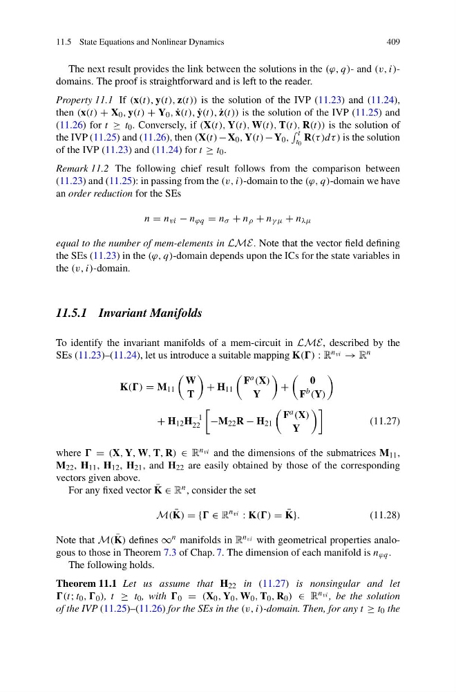
SEs (11.23)–(11.24), let us introduce a suitable mapping K() : R n vi → R n
K() = M 11
W
T
+ H 11
F a (X)
Y
+
0
F b (Y)
+ H 12 H
−1
22
−M 22 R − H 21
F a (X)
Y
(11.27)
where = (X, Y, W, T, R) ∈ R n vi and the dimensions of the submatrices M 11 ,
M 22 , H 11 , H 12 , H 21 , and H 22 are easily obtained by those of the corresponding
vectors given above.
For any fixed vector ¯
K ∈ R n , consider the set
M( ¯
K) = { ∈ R
n vi : K() = ¯
K}.
(11.28)
Note that M( ¯
K) defines ∞ n manifolds in R n vi with geometrical properties analogous to those in Theorem 7.3 of Chap. 7. The dimension of each manifold is n ϕq .
The following holds.
Theorem 11.1 Let us assume that H 22 in (11.27) is nonsingular and let
(t; t 0 , 0 ), t ≥ t 0 , with 0 = (X 0 , Y 0 , W 0 , T 0 , R 0 ) ∈ R n vi , be the solution
of the IVP (11.25)–(11.26) for the SEs in the (v, i)-domain. Then, for any t ≥ t 0 the
409
The next result provides the link between the solutions in the (ϕ, q)- and (v, i)domains. The proof is straightforward and is left to the reader.
Property 11.1 If (x(t), y(t), z(t)) is the solution of the IVP (11.23) and (11.24),
then (x(t) + X 0 , y(t) + Y 0 , ˙
x(t), ˙
y(t), ˙
z(t)) is the solution of the IVP (11.25) and
(11.26) for t ≥ t 0 . Conversely, if (X(t), Y(t), W(t), T(t), R(t)) is the solution of
the IVP (11.25) and (11.26), then (X(t) − X 0 , Y(t) − Y 0 ,
t
t 0
R(τ )dτ ) is the solution
of the IVP (11.23) and (11.24) for t ≥ t 0 .
Remark 11.2 The following chief result follows from the comparison between
(11.23) and (11.25): in passing from the (v, i)-domain to the (ϕ, q)-domain we have
an order reduction for the SEs
n = n vi − n ϕq = n σ + n ρ + n γ μ + n λμ
equal to the number of mem-elements in LME. Note that the vector field defining
the SEs (11.23) in the (ϕ, q)-domain depends upon the ICs for the state variables in
the (v, i)-domain.
11.5.1 Invariant Manifolds
To identify the invariant manifolds of a mem-circuit in LME, described by the
SEs (11.23)–(11.24), let us introduce a suitable mapping K() : R n vi → R n
K() = M 11
W
T
+ H 11
F a (X)
Y
+
0
F b (Y)
+ H 12 H
−1
22
−M 22 R − H 21
F a (X)
Y
(11.27)
where = (X, Y, W, T, R) ∈ R n vi and the dimensions of the submatrices M 11 ,
M 22 , H 11 , H 12 , H 21 , and H 22 are easily obtained by those of the corresponding
vectors given above.
For any fixed vector ¯
K ∈ R n , consider the set
M( ¯
K) = { ∈ R
n vi : K() = ¯
K}.
(11.28)
Note that M( ¯
K) defines ∞ n manifolds in R n vi with geometrical properties analogous to those in Theorem 7.3 of Chap. 7. The dimension of each manifold is n ϕq .
The following holds.
Theorem 11.1 Let us assume that H 22 in (11.27) is nonsingular and let
(t; t 0 , 0 ), t ≥ t 0 , with 0 = (X 0 , Y 0 , W 0 , T 0 , R 0 ) ∈ R n vi , be the solution
of the IVP (11.25)–(11.26) for the SEs in the (v, i)-domain. Then, for any t ≥ t 0 the