

370
9 Memristor Cellular Neural Networks Computing in the Flux-charge Domain
states, so that the dynamic analysis can be performed via a dynamic route map for a
first-order neuron. In the second case, an analog behavior with smooth memristance
changes is considered resulting in a true second-order dynamics. The behavior is
studied via an extended form of dynamic route map that can be applied to secondorder nonlinear dynamical systems.
Such papers stress that the unique capability of a nonvolatile resistance switching
memory to store or process data in the same physical nano-scale volume may be
leveraged in such CNNs to improve the performance of sensor-processor systems,
especially the spatial resolution of state-of-the-art visual microprocessors consisting
of Cellular Nonlinear Network computing machines [28] integrated on top of CMOS
image sensor arrays. The maximum number of smart sensors in these hardware
components is currently limited by the excessive integrated circuit area consumed
by each processing element, due to the need to accommodate large memory units
allowing to reprogram its circuit parameters as well as to store computation results
or to retrieve them at a later stage for further data processing. Relevant advantages
are potentially obtained, allowing to resolve the spatial resolution issue of modern
sensor-processor arrays, thanks to the capability to store and retrieve data into and
from the resistance switching memories without the necessity to reserve additional
cell circuit area for memory banks.
Appendix: HP Memristor with Joglekar Window
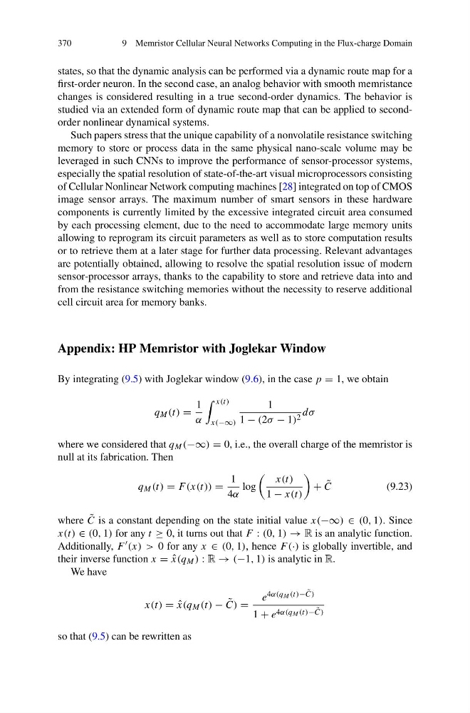
By integrating (9.5) with Joglekar window (9.6), in the case p = 1, we obtain
q M (t) =
1
α
x(t)
x(−∞)
1
1 − (2σ − 1) 2 dσ
where we considered that q M (−∞) = 0, i.e., the overall charge of the memristor is
null at its fabrication. Then
q M (t) = F (x(t)) =
1
4α
log
x(t)
1 − x(t)
+ ˜
C
(9.23)
where ˜
C is a constant depending on the state initial value x(−∞) ∈ (0, 1). Since
x(t) ∈ (0, 1) for any t ≥ 0, it turns out that F : (0, 1) → R is an analytic function.
Additionally, F (x) > 0 for any x ∈ (0, 1), hence F (·) is globally invertible, and
their inverse function x = ˆ
x(q M ) : R → (−1, 1) is analytic in R.
We have
x(t) = ˆ
x(q M (t) − ˜
C) =
e 4α(q M (t)− ˜
C)
1 + e 4α(q M (t)− ˜
C)
so that (9.5) can be rewritten as
9 Memristor Cellular Neural Networks Computing in the Flux-charge Domain
states, so that the dynamic analysis can be performed via a dynamic route map for a
first-order neuron. In the second case, an analog behavior with smooth memristance
changes is considered resulting in a true second-order dynamics. The behavior is
studied via an extended form of dynamic route map that can be applied to secondorder nonlinear dynamical systems.
Such papers stress that the unique capability of a nonvolatile resistance switching
memory to store or process data in the same physical nano-scale volume may be
leveraged in such CNNs to improve the performance of sensor-processor systems,
especially the spatial resolution of state-of-the-art visual microprocessors consisting
of Cellular Nonlinear Network computing machines [28] integrated on top of CMOS
image sensor arrays. The maximum number of smart sensors in these hardware
components is currently limited by the excessive integrated circuit area consumed
by each processing element, due to the need to accommodate large memory units
allowing to reprogram its circuit parameters as well as to store computation results
or to retrieve them at a later stage for further data processing. Relevant advantages
are potentially obtained, allowing to resolve the spatial resolution issue of modern
sensor-processor arrays, thanks to the capability to store and retrieve data into and
from the resistance switching memories without the necessity to reserve additional
cell circuit area for memory banks.
Appendix: HP Memristor with Joglekar Window
By integrating (9.5) with Joglekar window (9.6), in the case p = 1, we obtain
q M (t) =
1
α
x(t)
x(−∞)
1
1 − (2σ − 1) 2 dσ
where we considered that q M (−∞) = 0, i.e., the overall charge of the memristor is
null at its fabrication. Then
q M (t) = F (x(t)) =
1
4α
log
x(t)
1 − x(t)
+ ˜
C
(9.23)
where ˜
C is a constant depending on the state initial value x(−∞) ∈ (0, 1). Since
x(t) ∈ (0, 1) for any t ≥ 0, it turns out that F : (0, 1) → R is an analytic function.
Additionally, F (x) > 0 for any x ∈ (0, 1), hence F (·) is globally invertible, and
their inverse function x = ˆ
x(q M ) : R → (−1, 1) is analytic in R.
We have
x(t) = ˆ
x(q M (t) − ˜
C) =
e 4α(q M (t)− ˜
C)
1 + e 4α(q M (t)− ˜
C)
so that (9.5) can be rewritten as