

9.4 Applications to Image Processing
363
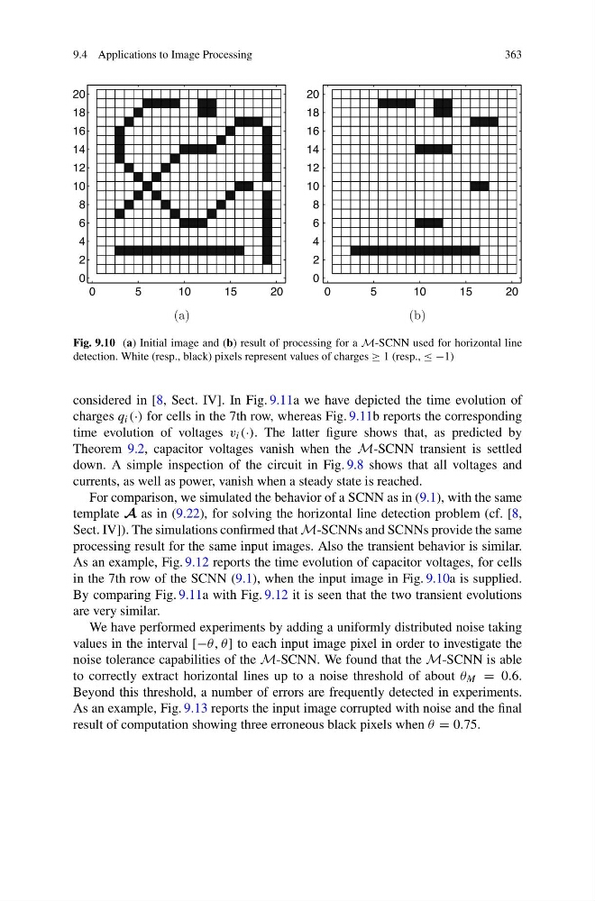
Fig. 9.10 (a) Initial image and (b) result of processing for a M-SCNN used for horizontal line
detection. White (resp., black) pixels represent values of charges ≥ 1 (resp., ≤ −1)
considered in [8, Sect. IV]. In Fig. 9.11a we have depicted the time evolution of
charges q i (·) for cells in the 7th row, whereas Fig. 9.11b reports the corresponding
time evolution of voltages v i (·). The latter figure shows that, as predicted by
Theorem 9.2, capacitor voltages vanish when the M-SCNN transient is settled
down. A simple inspection of the circuit in Fig. 9.8 shows that all voltages and
currents, as well as power, vanish when a steady state is reached.
For comparison, we simulated the behavior of a SCNN as in (9.1), with the same
template A as in (9.22), for solving the horizontal line detection problem (cf. [8,
Sect. IV]). The simulations confirmed that M-SCNNs and SCNNs provide the same
processing result for the same input images. Also the transient behavior is similar.
As an example, Fig. 9.12 reports the time evolution of capacitor voltages, for cells
in the 7th row of the SCNN (9.1), when the input image in Fig. 9.10a is supplied.
By comparing Fig. 9.11a with Fig. 9.12 it is seen that the two transient evolutions
are very similar.
We have performed experiments by adding a uniformly distributed noise taking
values in the interval [−θ, θ] to each input image pixel in order to investigate the
noise tolerance capabilities of the M-SCNN. We found that the M-SCNN is able
to correctly extract horizontal lines up to a noise threshold of about θ M = 0.6.
Beyond this threshold, a number of errors are frequently detected in experiments.
As an example, Fig. 9.13 reports the input image corrupted with noise and the final
result of computation showing three erroneous black pixels when θ = 0.75.
363
Fig. 9.10 (a) Initial image and (b) result of processing for a M-SCNN used for horizontal line
detection. White (resp., black) pixels represent values of charges ≥ 1 (resp., ≤ −1)
considered in [8, Sect. IV]. In Fig. 9.11a we have depicted the time evolution of
charges q i (·) for cells in the 7th row, whereas Fig. 9.11b reports the corresponding
time evolution of voltages v i (·). The latter figure shows that, as predicted by
Theorem 9.2, capacitor voltages vanish when the M-SCNN transient is settled
down. A simple inspection of the circuit in Fig. 9.8 shows that all voltages and
currents, as well as power, vanish when a steady state is reached.
For comparison, we simulated the behavior of a SCNN as in (9.1), with the same
template A as in (9.22), for solving the horizontal line detection problem (cf. [8,
Sect. IV]). The simulations confirmed that M-SCNNs and SCNNs provide the same
processing result for the same input images. Also the transient behavior is similar.
As an example, Fig. 9.12 reports the time evolution of capacitor voltages, for cells
in the 7th row of the SCNN (9.1), when the input image in Fig. 9.10a is supplied.
By comparing Fig. 9.11a with Fig. 9.12 it is seen that the two transient evolutions
are very similar.
We have performed experiments by adding a uniformly distributed noise taking
values in the interval [−θ, θ] to each input image pixel in order to investigate the
noise tolerance capabilities of the M-SCNN. We found that the M-SCNN is able
to correctly extract horizontal lines up to a noise threshold of about θ M = 0.6.
Beyond this threshold, a number of errors are frequently detected in experiments.
As an example, Fig. 9.13 reports the input image corrupted with noise and the final
result of computation showing three erroneous black pixels when θ = 0.75.