

362
9 Memristor Cellular Neural Networks Computing in the Flux-charge Domain
9.4.1 Horizontal Line Detection
In order to illustrate how the dynamics in the (ϕ, q)-domain of a convergent MSCNN can be used for processing purposes, let us consider a specific application
where a 2D M-SCNN array is used for extracting the horizontal lines of an image.
After reordering cells row-wise the M-SCNN can be described in the (ϕ, q)-domain
by the set of differential equations (9.13) and in the (v, i)-domain by (9.21).
According to Theorem 9.2, in a convergent M-SCNN all voltages and currents
vanish in steady state, so that the network cannot compute in the standard (v, i)domain. However, it can perform a processing in the (ϕ, q)-domain via the transient
dynamics of system (9.13). More precisely, first we design the interconnections of a
M-SCNN in order that the assumptions of Theorem 9.1 are satisfied, in particular,
we choose a symmetric matrix G. The input image to be processed is provided to the
M-SCNN (9.13) via the initial conditions q(0) = q 0 , the processing is performed
during the time evolution of the charges q(·) in (9.13) and the processing result is
given by the asymptotic values of the charges q(∞) = lim t→+∞ q(t).
For the horizontal line detection suppose to choose the same 3 × 3 feedback
cloning template as in [15, Sect. III]
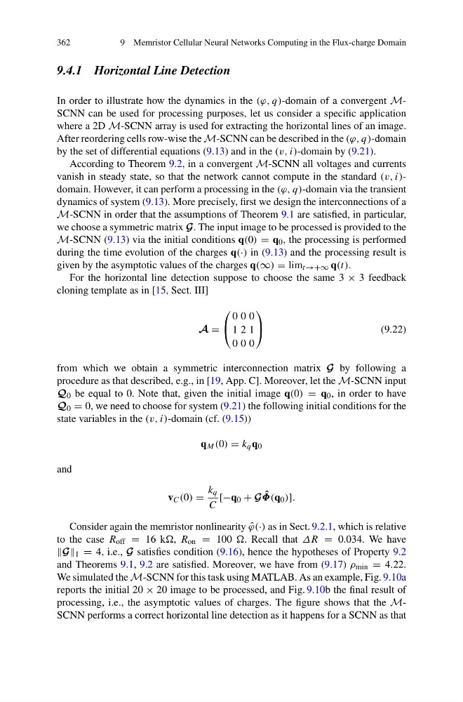
A =
⎛
⎝
0 0 0
1 2 1
0 0 0
⎞
⎠
(9.22)
from which we obtain a symmetric interconnection matrix G by following a
procedure as that described, e.g., in [19, App. C]. Moreover, let the M-SCNN input
Q 0 be equal to 0. Note that, given the initial image q(0) = q 0 , in order to have
Q 0 = 0, we need to choose for system (9.21) the following initial conditions for the
state variables in the (v, i)-domain (cf. (9.15))
q M (0) = k q q 0
and
v C (0) =
k q
C
[−q 0 + G ˆ
Φ(q 0 )].
Consider again the memristor nonlinearity ˆ
ϕ(·) as in Sect. 9.2.1, which is relative
to the case R off = 16 k, R on = 100 . Recall that ΔR = 0.034. We have
G 1 = 4, i.e., G satisfies condition (9.16), hence the hypotheses of Property 9.2
and Theorems 9.1, 9.2 are satisfied. Moreover, we have from (9.17) ρ min = 4.22.
We simulated the M-SCNN for this task using MATLAB. As an example, Fig. 9.10a
reports the initial 20 × 20 image to be processed, and Fig. 9.10b the final result of
processing, i.e., the asymptotic values of charges. The figure shows that the MSCNN performs a correct horizontal line detection as it happens for a SCNN as that
9 Memristor Cellular Neural Networks Computing in the Flux-charge Domain
9.4.1 Horizontal Line Detection
In order to illustrate how the dynamics in the (ϕ, q)-domain of a convergent MSCNN can be used for processing purposes, let us consider a specific application
where a 2D M-SCNN array is used for extracting the horizontal lines of an image.
After reordering cells row-wise the M-SCNN can be described in the (ϕ, q)-domain
by the set of differential equations (9.13) and in the (v, i)-domain by (9.21).
According to Theorem 9.2, in a convergent M-SCNN all voltages and currents
vanish in steady state, so that the network cannot compute in the standard (v, i)domain. However, it can perform a processing in the (ϕ, q)-domain via the transient
dynamics of system (9.13). More precisely, first we design the interconnections of a
M-SCNN in order that the assumptions of Theorem 9.1 are satisfied, in particular,
we choose a symmetric matrix G. The input image to be processed is provided to the
M-SCNN (9.13) via the initial conditions q(0) = q 0 , the processing is performed
during the time evolution of the charges q(·) in (9.13) and the processing result is
given by the asymptotic values of the charges q(∞) = lim t→+∞ q(t).
For the horizontal line detection suppose to choose the same 3 × 3 feedback
cloning template as in [15, Sect. III]
A =
⎛
⎝
0 0 0
1 2 1
0 0 0
⎞
⎠
(9.22)
from which we obtain a symmetric interconnection matrix G by following a
procedure as that described, e.g., in [19, App. C]. Moreover, let the M-SCNN input
Q 0 be equal to 0. Note that, given the initial image q(0) = q 0 , in order to have
Q 0 = 0, we need to choose for system (9.21) the following initial conditions for the
state variables in the (v, i)-domain (cf. (9.15))
q M (0) = k q q 0
and
v C (0) =
k q
C
[−q 0 + G ˆ
Φ(q 0 )].
Consider again the memristor nonlinearity ˆ
ϕ(·) as in Sect. 9.2.1, which is relative
to the case R off = 16 k, R on = 100 . Recall that ΔR = 0.034. We have
G 1 = 4, i.e., G satisfies condition (9.16), hence the hypotheses of Property 9.2
and Theorems 9.1, 9.2 are satisfied. Moreover, we have from (9.17) ρ min = 4.22.
We simulated the M-SCNN for this task using MATLAB. As an example, Fig. 9.10a
reports the initial 20 × 20 image to be processed, and Fig. 9.10b the final result of
processing, i.e., the asymptotic values of charges. The figure shows that the MSCNN performs a correct horizontal line detection as it happens for a SCNN as that