

9.2 Memristor Neural Network Model
347
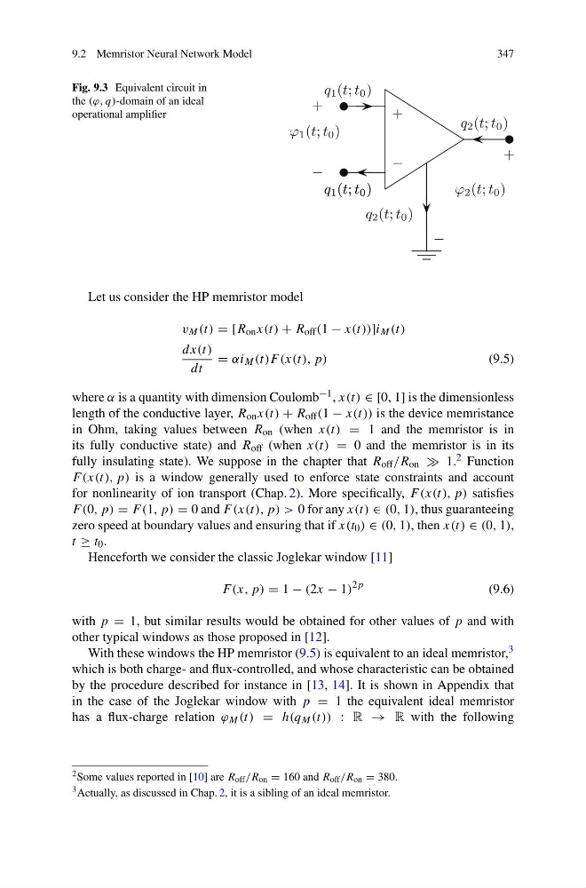
Fig. 9.3 Equivalent circuit in
the (ϕ, q)-domain of an ideal
operational amplifier
Let us consider the HP memristor model
v M (t) = [R on x(t) + R off (1 − x(t))]i M (t)
dx(t)
dt
= αi M (t)F (x(t), p)
(9.5)
where α is a quantity with dimension Coulomb −1 , x(t) ∈ [0, 1] is the dimensionless
length of the conductive layer, R on x(t) + R off (1 − x(t)) is the device memristance
in Ohm, taking values between R on (when x(t) = 1 and the memristor is in
its fully conductive state) and R off (when x(t) = 0 and the memristor is in its
fully insulating state). We suppose in the chapter that R off /R on 1. 2 Function
F (x(t), p) is a window generally used to enforce state constraints and account
for nonlinearity of ion transport (Chap. 2). More specifically, F (x(t), p) satisfies
F (0, p) = F (1, p) = 0 and F (x(t), p) > 0 for any x(t) ∈ (0, 1), thus guaranteeing
zero speed at boundary values and ensuring that if x(t 0 ) ∈ (0, 1), then x(t) ∈ (0, 1),
t ≥ t 0 .
Henceforth we consider the classic Joglekar window [11]
F (x, p) = 1 − (2x − 1)
2p
(9.6)
with p = 1, but similar results would be obtained for other values of p and with
other typical windows as those proposed in [12].
With these windows the HP memristor (9.5) is equivalent to an ideal memristor, 3
which is both charge- and flux-controlled, and whose characteristic can be obtained
by the procedure described for instance in [13, 14]. It is shown in Appendix that
in the case of the Joglekar window with p = 1 the equivalent ideal memristor
has a flux-charge relation ϕ M (t) = h(q M (t)) : R → R with the following
2 Some values reported in [10] are R off /R on = 160 and R off /R on = 380.
3 Actually, as discussed in Chap. 2, it is a sibling of an ideal memristor.
347
Fig. 9.3 Equivalent circuit in
the (ϕ, q)-domain of an ideal
operational amplifier
Let us consider the HP memristor model
v M (t) = [R on x(t) + R off (1 − x(t))]i M (t)
dx(t)
dt
= αi M (t)F (x(t), p)
(9.5)
where α is a quantity with dimension Coulomb −1 , x(t) ∈ [0, 1] is the dimensionless
length of the conductive layer, R on x(t) + R off (1 − x(t)) is the device memristance
in Ohm, taking values between R on (when x(t) = 1 and the memristor is in
its fully conductive state) and R off (when x(t) = 0 and the memristor is in its
fully insulating state). We suppose in the chapter that R off /R on 1. 2 Function
F (x(t), p) is a window generally used to enforce state constraints and account
for nonlinearity of ion transport (Chap. 2). More specifically, F (x(t), p) satisfies
F (0, p) = F (1, p) = 0 and F (x(t), p) > 0 for any x(t) ∈ (0, 1), thus guaranteeing
zero speed at boundary values and ensuring that if x(t 0 ) ∈ (0, 1), then x(t) ∈ (0, 1),
t ≥ t 0 .
Henceforth we consider the classic Joglekar window [11]
F (x, p) = 1 − (2x − 1)
2p
(9.6)
with p = 1, but similar results would be obtained for other values of p and with
other typical windows as those proposed in [12].
With these windows the HP memristor (9.5) is equivalent to an ideal memristor, 3
which is both charge- and flux-controlled, and whose characteristic can be obtained
by the procedure described for instance in [13, 14]. It is shown in Appendix that
in the case of the Joglekar window with p = 1 the equivalent ideal memristor
has a flux-charge relation ϕ M (t) = h(q M (t)) : R → R with the following
2 Some values reported in [10] are R off /R on = 160 and R off /R on = 380.
3 Actually, as discussed in Chap. 2, it is a sibling of an ideal memristor.