

9.2 Memristor Neural Network Model
345
9.2 Memristor Neural Network Model
The equations describing in the (v, i)-domain the dynamics of the SCNN model [8]
can be written in matrix-vector form as follows:
C
dv(t)
dt
= −
v(t)
R
+ GS(v(t)) + I
(9.1)
where C and R are the cell capacitor and resistor, respectively, v(t) ∈ R n is the
vector of capacitor voltages, G ∈ R n×n is the interconnection matrix, and I ∈ R n is a
biasing input. Moreover, S(v(t)) = (s(v 1 (t)), s(v 2 (t)), . . . , s(v n (t))) T : R n → R n ,
where
s(ρ) =
1
2
(|ρ + 1| − |ρ − 1|)
(9.2)
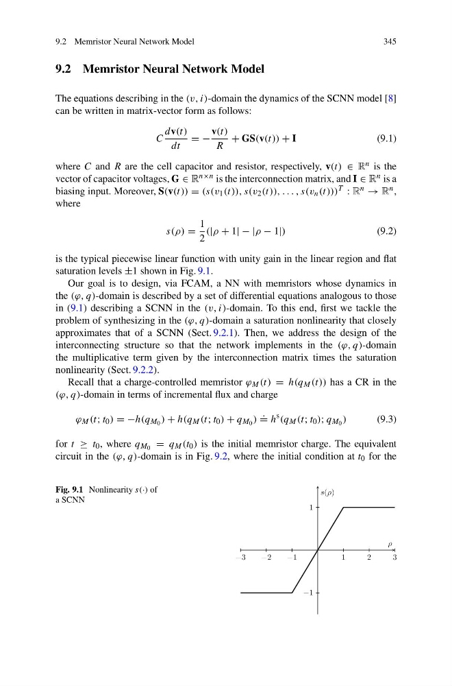
is the typical piecewise linear function with unity gain in the linear region and flat
saturation levels ±1 shown in Fig. 9.1.
Our goal is to design, via FCAM, a NN with memristors whose dynamics in
the (ϕ, q)-domain is described by a set of differential equations analogous to those
in (9.1) describing a SCNN in the (v, i)-domain. To this end, first we tackle the
problem of synthesizing in the (ϕ, q)-domain a saturation nonlinearity that closely
approximates that of a SCNN (Sect. 9.2.1). Then, we address the design of the
interconnecting structure so that the network implements in the (ϕ, q)-domain
the multiplicative term given by the interconnection matrix times the saturation
nonlinearity (Sect. 9.2.2).
Recall that a charge-controlled memristor ϕ M (t) = h(q M (t)) has a CR in the
(ϕ, q)-domain in terms of incremental flux and charge
ϕ M (t; t 0 ) = −h(q M 0 ) + h(q M (t; t 0 ) + q M 0 )
.
= h
s (q M (t; t 0 ); q M 0 )
(9.3)
for t ≥ t 0 , where q M 0 = q M (t 0 ) is the initial memristor charge. The equivalent
circuit in the (ϕ, q)-domain is in Fig. 9.2, where the initial condition at t 0 for the
Fig. 9.1 Nonlinearity s(·) of
a SCNN
345
9.2 Memristor Neural Network Model
The equations describing in the (v, i)-domain the dynamics of the SCNN model [8]
can be written in matrix-vector form as follows:
C
dv(t)
dt
= −
v(t)
R
+ GS(v(t)) + I
(9.1)
where C and R are the cell capacitor and resistor, respectively, v(t) ∈ R n is the
vector of capacitor voltages, G ∈ R n×n is the interconnection matrix, and I ∈ R n is a
biasing input. Moreover, S(v(t)) = (s(v 1 (t)), s(v 2 (t)), . . . , s(v n (t))) T : R n → R n ,
where
s(ρ) =
1
2
(|ρ + 1| − |ρ − 1|)
(9.2)
is the typical piecewise linear function with unity gain in the linear region and flat
saturation levels ±1 shown in Fig. 9.1.
Our goal is to design, via FCAM, a NN with memristors whose dynamics in
the (ϕ, q)-domain is described by a set of differential equations analogous to those
in (9.1) describing a SCNN in the (v, i)-domain. To this end, first we tackle the
problem of synthesizing in the (ϕ, q)-domain a saturation nonlinearity that closely
approximates that of a SCNN (Sect. 9.2.1). Then, we address the design of the
interconnecting structure so that the network implements in the (ϕ, q)-domain
the multiplicative term given by the interconnection matrix times the saturation
nonlinearity (Sect. 9.2.2).
Recall that a charge-controlled memristor ϕ M (t) = h(q M (t)) has a CR in the
(ϕ, q)-domain in terms of incremental flux and charge
ϕ M (t; t 0 ) = −h(q M 0 ) + h(q M (t; t 0 ) + q M 0 )
.
= h
s (q M (t; t 0 ); q M 0 )
(9.3)
for t ≥ t 0 , where q M 0 = q M (t 0 ) is the initial memristor charge. The equivalent
circuit in the (ϕ, q)-domain is in Fig. 9.2, where the initial condition at t 0 for the
Fig. 9.1 Nonlinearity s(·) of
a SCNN