

6
1 Device Modeling and Circuit Elements
A circuit element defined mathematically by a CR should ideally display
the same qualitative behavior that a device D exhibits when connected to an
excitation network and it should have predictive ability, i.e., it should be capable
of predicting previously unknown operating modes through computer simulation.
Readers interested in a detailed discussion of the main qualitative properties (e.g.,
well-posedness, simulation capability, qualitative similarity, predictive ability, and
structural stability) that a circuit model of a device D should possess can refer to the
fundamental article [1].
The mathematical equations describing a circuit element are in general nonlinear and may include a combination of algebraic equations, ordinary differential
equations, partial differential equations, and integral equations. A two-terminal
circuit element is said to be lumped if and only if its CR can be expressed by a
finite number of equations involving only algebraic, ordinary differentiation, and
integration operations on the instantaneous values of the terminal variables {v, i}
and/or a finite number of additional internal variables {x 1 , x 2 , . . . , x n }. Otherwise,
the two-terminal circuit element is said to be distributed.
From now on the book is concerned with lumped circuit elements only. The
CR of a lumped circuit element may involve not only v(t) and i(t) but also their
higher-order derivatives and integrals defined recursively as follows for any integers
α and β.
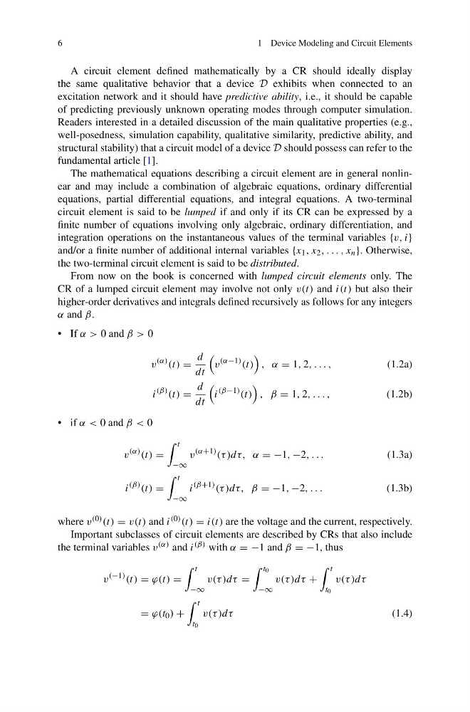
• If α > 0 and β > 0
v
(α) (t) =
d
dt
v
(α−1) (t)
, α = 1, 2, . . . ,
(1.2a)
i
(β) (t) =
d
dt
i
(β−1) (t)
, β = 1, 2, . . . ,
(1.2b)
• if α < 0 and β < 0
v
(α) (t) =
t
−∞
v
(α+1) (τ )dτ, α = −1, −2, . . .
(1.3a)
i
(β) (t) =
t
−∞
i
(β+1) (τ )dτ, β = −1, −2, . . .
(1.3b)
where v (0) (t) = v(t) and i (0) (t) = i(t) are the voltage and the current, respectively.
Important subclasses of circuit elements are described by CRs that also include
the terminal variables v (α) and i (β) with α = −1 and β = −1, thus
v
(−1) (t) = ϕ(t) =
t
−∞
v(τ )dτ =
t 0
−∞
v(τ )dτ +
t
t 0
v(τ )dτ
= ϕ(t 0 ) +
t
t 0
v(τ )dτ
(1.4)
1 Device Modeling and Circuit Elements
A circuit element defined mathematically by a CR should ideally display
the same qualitative behavior that a device D exhibits when connected to an
excitation network and it should have predictive ability, i.e., it should be capable
of predicting previously unknown operating modes through computer simulation.
Readers interested in a detailed discussion of the main qualitative properties (e.g.,
well-posedness, simulation capability, qualitative similarity, predictive ability, and
structural stability) that a circuit model of a device D should possess can refer to the
fundamental article [1].
The mathematical equations describing a circuit element are in general nonlinear and may include a combination of algebraic equations, ordinary differential
equations, partial differential equations, and integral equations. A two-terminal
circuit element is said to be lumped if and only if its CR can be expressed by a
finite number of equations involving only algebraic, ordinary differentiation, and
integration operations on the instantaneous values of the terminal variables {v, i}
and/or a finite number of additional internal variables {x 1 , x 2 , . . . , x n }. Otherwise,
the two-terminal circuit element is said to be distributed.
From now on the book is concerned with lumped circuit elements only. The
CR of a lumped circuit element may involve not only v(t) and i(t) but also their
higher-order derivatives and integrals defined recursively as follows for any integers
α and β.
• If α > 0 and β > 0
v
(α) (t) =
d
dt
v
(α−1) (t)
, α = 1, 2, . . . ,
(1.2a)
i
(β) (t) =
d
dt
i
(β−1) (t)
, β = 1, 2, . . . ,
(1.2b)
• if α < 0 and β < 0
v
(α) (t) =
t
−∞
v
(α+1) (τ )dτ, α = −1, −2, . . .
(1.3a)
i
(β) (t) =
t
−∞
i
(β+1) (τ )dτ, β = −1, −2, . . .
(1.3b)
where v (0) (t) = v(t) and i (0) (t) = i(t) are the voltage and the current, respectively.
Important subclasses of circuit elements are described by CRs that also include
the terminal variables v (α) and i (β) with α = −1 and β = −1, thus
v
(−1) (t) = ϕ(t) =
t
−∞
v(τ )dτ =
t 0
−∞
v(τ )dτ +
t
t 0
v(τ )dτ
= ϕ(t 0 ) +
t
t 0
v(τ )dτ
(1.4)