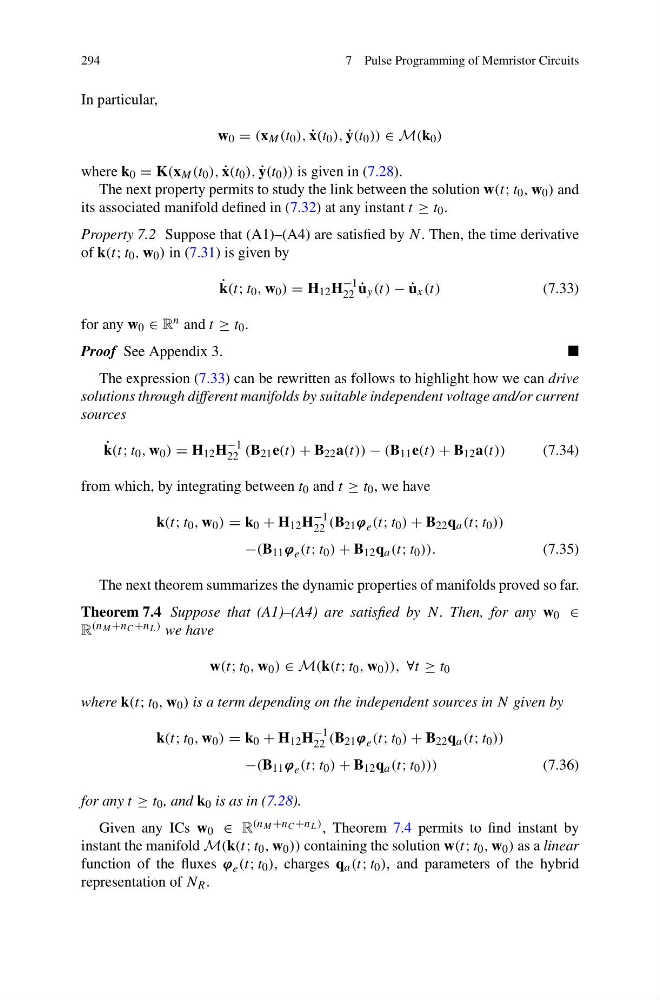
294
7 Pulse Programming of Memristor Circuits
In particular,
w 0 = (x M (t 0 ), ˙
x(t 0 ), ˙
y(t 0 )) ∈ M(k 0 )
where k 0 = K(x M (t 0 ), ˙
x(t 0 ), ˙
y(t 0 )) is given in (7.28).
The next property permits to study the link between the solution w(t; t 0 , w 0 ) and
its associated manifold defined in (7.32) at any instant t ≥ t 0 .
Property 7.2 Suppose that (A1)–(A4) are satisfied by N . Then, the time derivative
of k(t; t 0 , w 0 ) in (7.31) is given by
˙
k(t; t 0 , w 0 ) = H 12 H
−1
22 ˙
u y (t) − ˙
u x (t)
(7.33)
for any w 0 ∈ R n and t ≥ t 0 .
Proof See Appendix 3.
The expression (7.33) can be rewritten as follows to highlight how we can drive
solutions through different manifolds by suitable independent voltage and/or current
sources
˙
k(t; t 0 , w 0 ) = H 12 H
−1
22 (B 21 e(t) + B 22 a(t)) − (B 11 e(t) + B 12 a(t))
(7.34)
from which, by integrating between t 0 and t ≥ t 0 , we have
k(t; t 0 , w 0 ) = k 0 + H 12 H
−1
22 (B 21 ϕ e (t; t 0 ) + B 22 q a (t; t 0 ))
−(B 11 ϕ e (t; t 0 ) + B 12 q a (t; t 0 )).
(7.35)
The next theorem summarizes the dynamic properties of manifolds proved so far.
Theorem 7.4 Suppose that (A1)–(A4) are satisfied by N . Then, for any w 0 ∈
R (n M +n C +n L ) we have
w(t; t 0 , w 0 ) ∈ M(k(t; t 0 , w 0 )), ∀t ≥ t 0
where k(t; t 0 , w 0 ) is a term depending on the independent sources in N given by
k(t; t 0 , w 0 ) = k 0 + H 12 H
−1
22 (B 21 ϕ e (t; t 0 ) + B 22 q a (t; t 0 ))
−(B 11 ϕ e (t; t 0 ) + B 12 q a (t; t 0 )))
(7.36)
for any t ≥ t 0 , and k 0 is as in (7.28).
Given any ICs w 0 ∈ R (n M +n C +n L ) , Theorem 7.4 permits to find instant by
instant the manifold M(k(t; t 0 , w 0 )) containing the solution w(t; t 0 , w 0 ) as a linear
function of the fluxes ϕ e (t; t 0 ), charges q a (t; t 0 ), and parameters of the hybrid
representation of N R .