

228
6 Memristor Circuits: Invariant Manifolds, Coexisting Attractors, Extreme. . .
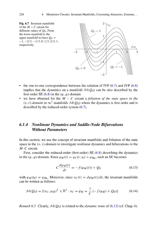
Fig. 6.7 Invariant manifolds
of the M − C circuit for
different values of Q 0 . From
the lower manifold to the
upper manifold we have Q 0 =
−1, −2/3, −1/3, 0, 1/3, 2/3, 1,
respectively
−3
−2
−1
1
2
3
−2
−1
1
2
Q 0 = −1
Q 0 = 1
Q 0 = 0
ϕ M
v C
• the one-to-one correspondence between the solution of IVP (6.7) and IVP (6.8)
implies that the dynamics on a manifold M(Q 0 ) can be also described by the
first-order SE (6.8) in the (ϕ, q)-domain
• we have obtained for the M − C circuit a foliation of the state space in the
(v, i)-domain in ∞ 1 manifolds M(Q 0 ) where the dynamics is first order and is
described by the reduced-order system (6.7).
6.1.4 Nonlinear Dynamics and Saddle-Node Bifurcations
Without Parameters
In this section, we use the concept of invariant manifolds and foliation of the state
space in the (v, i)-domain to investigate nonlinear dynamics and bifurcations in the
M–C circuit.
First, consider the reduced-order (first-order) SE (6.8) describing the dynamics
in the (ϕ, q)-domain. Since ϕ M (t) = ϕ C (t; t 0 ) + ϕ M 0 , such an SE becomes
C
dϕ M (t)
dt
= −f (ϕ M (t)) + Q 0
(6.13)
with ϕ M (t 0 ) = ϕ M 0 . Moreover, since v C (t) = dϕ M (t)/dt, the invariant manifolds
can be written as follows:
M(Q 0 ) = {(v C , ϕ M )
T
∈ R
2
: v C = ˙
ϕ M =
1
C
(−f (ϕ M ) + Q 0 )}.
(6.14)
Remark 6.5 Clearly, M(Q 0 ) is related to the dynamic route of (6.13) (cf. Chap. 4).
6 Memristor Circuits: Invariant Manifolds, Coexisting Attractors, Extreme. . .
Fig. 6.7 Invariant manifolds
of the M − C circuit for
different values of Q 0 . From
the lower manifold to the
upper manifold we have Q 0 =
−1, −2/3, −1/3, 0, 1/3, 2/3, 1,
respectively
−3
−2
−1
1
2
3
−2
−1
1
2
Q 0 = −1
Q 0 = 1
Q 0 = 0
ϕ M
v C
• the one-to-one correspondence between the solution of IVP (6.7) and IVP (6.8)
implies that the dynamics on a manifold M(Q 0 ) can be also described by the
first-order SE (6.8) in the (ϕ, q)-domain
• we have obtained for the M − C circuit a foliation of the state space in the
(v, i)-domain in ∞ 1 manifolds M(Q 0 ) where the dynamics is first order and is
described by the reduced-order system (6.7).
6.1.4 Nonlinear Dynamics and Saddle-Node Bifurcations
Without Parameters
In this section, we use the concept of invariant manifolds and foliation of the state
space in the (v, i)-domain to investigate nonlinear dynamics and bifurcations in the
M–C circuit.
First, consider the reduced-order (first-order) SE (6.8) describing the dynamics
in the (ϕ, q)-domain. Since ϕ M (t) = ϕ C (t; t 0 ) + ϕ M 0 , such an SE becomes
C
dϕ M (t)
dt
= −f (ϕ M (t)) + Q 0
(6.13)
with ϕ M (t 0 ) = ϕ M 0 . Moreover, since v C (t) = dϕ M (t)/dt, the invariant manifolds
can be written as follows:
M(Q 0 ) = {(v C , ϕ M )
T
∈ R
2
: v C = ˙
ϕ M =
1
C
(−f (ϕ M ) + Q 0 )}.
(6.14)
Remark 6.5 Clearly, M(Q 0 ) is related to the dynamic route of (6.13) (cf. Chap. 4).