

6.1 First-Order Memristor Circuits
225
6.1.2 M − C Circuit
The linear circuits studied in Sect. 6.1.1 illustrate the idea of foliation of the state
space, invariants of motion, invariants manifolds, and coexisting reduced-order
dynamics. However, due to the linearity, each reduced-order dynamics has the
same properties from a stability viewpoint and there are no bifurcations when
changing the initial conditions for fixed circuit parameters. As shown next, there is
a radical change from the viewpoint of stability and bifurcations when we consider
a nonlinear memristor circuit.
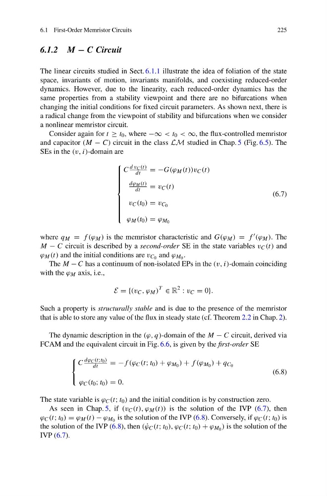
Consider again for t ≥ t 0 , where −∞ < t 0 < ∞, the flux-controlled memristor
and capacitor (M − C) circuit in the class LM studied in Chap. 5 (Fig. 6.5). The
SEs in the (v, i)-domain are
⎧
⎪ ⎪ ⎪ ⎪ ⎪ ⎪ ⎪ ⎨
⎪ ⎪ ⎪ ⎪ ⎪ ⎪ ⎪ ⎩
C
d v C (t)
dt
= −G(ϕ M (t))v C (t)
dϕ M (t)
dt
= v C (t)
v C (t 0 ) = v C 0
ϕ M (t 0 ) = ϕ M 0
(6.7)
where q M = f (ϕ M ) is the memristor characteristic and G(ϕ M ) = f (ϕ M ). The
M − C circuit is described by a second-order SE in the state variables v C (t) and
ϕ M (t) and the initial conditions are v C 0 and ϕ M 0 .
The M − C has a continuum of non-isolated EPs in the (v, i)-domain coinciding
with the ϕ M axis, i.e.,
E = {(v C , ϕ M )
T
∈ R
2
: v C = 0}.
Such a property is structurally stable and is due to the presence of the memristor
that is able to store any value of the flux in steady state (cf. Theorem 2.2 in Chap. 2).
The dynamic description in the (ϕ, q)-domain of the M − C circuit, derived via
FCAM and the equivalent circuit in Fig. 6.6, is given by the first-order SE
⎧
⎨
⎩
C
dϕ C (t;t 0 )
dt
= −f (ϕ C (t; t 0 ) + ϕ M 0 ) + f (ϕ M 0 ) + q C 0
ϕ C (t 0 ; t 0 ) = 0.
(6.8)
The state variable is ϕ C (t; t 0 ) and the initial condition is by construction zero.
As seen in Chap. 5, if (v C (t), ϕ M (t)) is the solution of the IVP (6.7), then
ϕ C (t; t 0 ) = ϕ M (t) − ϕ M 0 is the solution of the IVP (6.8). Conversely, if ϕ C (t; t 0 ) is
the solution of the IVP (6.8), then ( ˙
ϕ C (t; t 0 ), ϕ C (t; t 0 ) + ϕ M 0 ) is the solution of the
IVP (6.7).
225
6.1.2 M − C Circuit
The linear circuits studied in Sect. 6.1.1 illustrate the idea of foliation of the state
space, invariants of motion, invariants manifolds, and coexisting reduced-order
dynamics. However, due to the linearity, each reduced-order dynamics has the
same properties from a stability viewpoint and there are no bifurcations when
changing the initial conditions for fixed circuit parameters. As shown next, there is
a radical change from the viewpoint of stability and bifurcations when we consider
a nonlinear memristor circuit.
Consider again for t ≥ t 0 , where −∞ < t 0 < ∞, the flux-controlled memristor
and capacitor (M − C) circuit in the class LM studied in Chap. 5 (Fig. 6.5). The
SEs in the (v, i)-domain are
⎧
⎪ ⎪ ⎪ ⎪ ⎪ ⎪ ⎪ ⎨
⎪ ⎪ ⎪ ⎪ ⎪ ⎪ ⎪ ⎩
C
d v C (t)
dt
= −G(ϕ M (t))v C (t)
dϕ M (t)
dt
= v C (t)
v C (t 0 ) = v C 0
ϕ M (t 0 ) = ϕ M 0
(6.7)
where q M = f (ϕ M ) is the memristor characteristic and G(ϕ M ) = f (ϕ M ). The
M − C circuit is described by a second-order SE in the state variables v C (t) and
ϕ M (t) and the initial conditions are v C 0 and ϕ M 0 .
The M − C has a continuum of non-isolated EPs in the (v, i)-domain coinciding
with the ϕ M axis, i.e.,
E = {(v C , ϕ M )
T
∈ R
2
: v C = 0}.
Such a property is structurally stable and is due to the presence of the memristor
that is able to store any value of the flux in steady state (cf. Theorem 2.2 in Chap. 2).
The dynamic description in the (ϕ, q)-domain of the M − C circuit, derived via
FCAM and the equivalent circuit in Fig. 6.6, is given by the first-order SE
⎧
⎨
⎩
C
dϕ C (t;t 0 )
dt
= −f (ϕ C (t; t 0 ) + ϕ M 0 ) + f (ϕ M 0 ) + q C 0
ϕ C (t 0 ; t 0 ) = 0.
(6.8)
The state variable is ϕ C (t; t 0 ) and the initial condition is by construction zero.
As seen in Chap. 5, if (v C (t), ϕ M (t)) is the solution of the IVP (6.7), then
ϕ C (t; t 0 ) = ϕ M (t) − ϕ M 0 is the solution of the IVP (6.8). Conversely, if ϕ C (t; t 0 ) is
the solution of the IVP (6.8), then ( ˙
ϕ C (t; t 0 ), ϕ C (t; t 0 ) + ϕ M 0 ) is the solution of the
IVP (6.7).