

6.1 First-Order Memristor Circuits
221
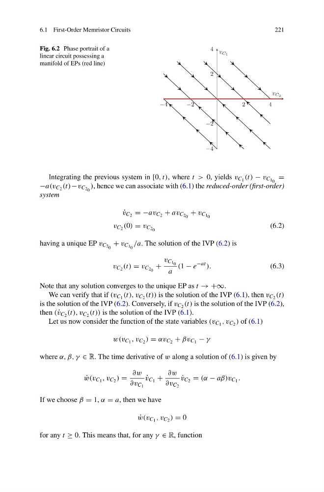
Fig. 6.2 Phase portrait of a
linear circuit possessing a
manifold of EPs (red line)
−4
−2
2
4
−4
−2
2
4
v C2
v C1
Integrating the previous system in [0, t), where t > 0, yields v C 1 (t) − v C 1 0 =
−a(v C 2 (t)−v C 2 0 ), hence we can associate with (6.1) the reduced-order (first-order)
system
˙
v C 2 = −av C 2 + av C 2 0 + v C 1 0
v C 2 (0) = v C 2 0
(6.2)
having a unique EP v C 2 0 + v C 1 0 /a. The solution of the IVP (6.2) is
v C 2 (t) = v C 2 0 +
v C 1 0
a
(1 − e
−at ).
(6.3)
Note that any solution converges to the unique EP as t → +∞.
We can verify that if (v C 1 (t), v C 2 (t)) is the solution of the IVP (6.1), then v C 2 (t)
is the solution of the IVP (6.2). Conversely, if v C 2 (t) is the solution of the IVP (6.2),
then ( ˙
v C 2 (t), v C 2 (t)) is the solution of the IVP (6.1).
Let us now consider the function of the state variables (v C 1 , v C 2 ) of (6.1)
w(v C 1 , v C 2 ) = αv C 2 + βv C 1 − γ
where α, β, γ ∈ R. The time derivative of w along a solution of (6.1) is given by
˙
w(v C 1 , v C 2 ) =
∂w
∂v C 1
˙
v C 1 +
∂w
∂v C 2
˙
v C 2 = (α − aβ)v C 1 .
If we choose β = 1, α = a, then we have
˙
w(v C 1 , v C 2 ) = 0
for any t ≥ 0. This means that, for any γ ∈ R, function
221
Fig. 6.2 Phase portrait of a
linear circuit possessing a
manifold of EPs (red line)
−4
−2
2
4
−4
−2
2
4
v C2
v C1
Integrating the previous system in [0, t), where t > 0, yields v C 1 (t) − v C 1 0 =
−a(v C 2 (t)−v C 2 0 ), hence we can associate with (6.1) the reduced-order (first-order)
system
˙
v C 2 = −av C 2 + av C 2 0 + v C 1 0
v C 2 (0) = v C 2 0
(6.2)
having a unique EP v C 2 0 + v C 1 0 /a. The solution of the IVP (6.2) is
v C 2 (t) = v C 2 0 +
v C 1 0
a
(1 − e
−at ).
(6.3)
Note that any solution converges to the unique EP as t → +∞.
We can verify that if (v C 1 (t), v C 2 (t)) is the solution of the IVP (6.1), then v C 2 (t)
is the solution of the IVP (6.2). Conversely, if v C 2 (t) is the solution of the IVP (6.2),
then ( ˙
v C 2 (t), v C 2 (t)) is the solution of the IVP (6.1).
Let us now consider the function of the state variables (v C 1 , v C 2 ) of (6.1)
w(v C 1 , v C 2 ) = αv C 2 + βv C 1 − γ
where α, β, γ ∈ R. The time derivative of w along a solution of (6.1) is given by
˙
w(v C 1 , v C 2 ) =
∂w
∂v C 1
˙
v C 1 +
∂w
∂v C 2
˙
v C 2 = (α − aβ)v C 1 .
If we choose β = 1, α = a, then we have
˙
w(v C 1 , v C 2 ) = 0
for any t ≥ 0. This means that, for any γ ∈ R, function